Contour Recursion and Auto-Segmentation
Aaron Carter-Ényì
KEYWORDS: contour theory, computational analysis, pitch perception, Schoenberg
ABSTRACT: Contour recursion, a pattern of ups and downs found at multiple indices in an ordinal pitch series, is proposed as a basis for melodic segmentation and a computational method. The continuous C+ matrix (CONTCOM) is introduced with a moving window of degrees of adjacency that accommodates analysis of unsegmented pitch series. CONTCOM converts an ordinal pitch series into contour slices in an abstraction of pitch space that uses contour levels instead of contour pitches. Using a CONTCOM, an algorithm implemented in MATLAB searches for recursive patterns, recognizes transformations, and compares segments of different cardinalities. An analysis of Schoenberg’s op. 19, no. 4 is offered as a demonstration of these methods.
Copyright © 2016 Society for Music Theory
1. Introduction
[1.1] Contour theory and analysis has a multi-disciplinary basis in music research with significant contributions from ethnomusicology(1), cognitive science(2), composition theory(3), music analysis(4), and music information retrieval.(5) The literature on melodic contour is unified by agreement that rises and falls in pitch are salient, but the type of comparisons made (local, global, or all possible) varies widely. The most promising application of contour analysis is comparing melodic segments that are perceptually similar (gestalt) but differ in interval content. Yet we lack formal criteria for picking out segments from musical works to draw comparisons.
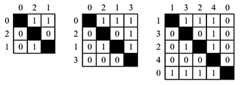
[1.2] One of the most useful tools for describing contour and measuring similarity is the COM-matrix introduced and formalized by Robert Morris in his 1987 book Composition with Pitch-Classes (see Figure 1). A COM-matrix is produced by making comparisons between all pitches in the segment up to the possible degrees of adjacency (from 1 to \(n-1\)). Two segments of the same cardinality (n), whether found or generated, are considered equivalent if they produce the same matrix and sum to the same CSEG. If not, a calculation of similarity can be made, called CSIM by Marvin and Laprade (1987). The COM-matrix, CSEG classes, and CSIM have limited utility in computational analysis because of the need for manual segmentation. A computer must be told where to look and what cardinality to use. The COM-matrix also has a rigid standard for equivalence (hence the need for CSIM) and does not accommodate comparing segments of different lengths. Furthermore, these tools are intended for highly varied pitch content and struggle with recurring pitches within a melodic segment, which are likely to be found in tonal and non-Western musics. These issues—(1) segmentation, (2) equivalence, (3) cardinality sensitivity, and (4) pitch multiplicity—have motivated revisions and alternative formulations by theorists including Robert Morris (who devised the COM-matrix), David Huron, Larry Polansky and Ian Quinn.
[1.3] Morris’s contour reduction algorithm (1993) provides a much less rigid form of equivalence and fully accommodates comparison of different cardinalities of contour segments. Through pruning all but time- and height-extreme contour pitches, CSEGs are reduced to a prime of two, three, or four elements. However, the algorithm still depends upon segmentation, and segments reduced to primes lose characteristics that may be important. Complexity is tracked through the assignment of a depth based on the number of passes necessary to reach prime form. Still, Morris’s algorithm continues to be a mainstay in music theory: it is central to recent dissertations by Schultz (2009), Bor (2009), and Sekula (2014), and Ohriner (2012) has applied it to rubato.
[1.4] A concurrent body of work on contour comes from computational (or systematic) musicology, and more recently music information retrieval (MIR). Huron offers operational concepts of similarity, not restricted to contour, that make it possible to “characterize degrees of resemblance” beyond “absolute matches” (2002, 21). The Humdrum Toolkit (1994) includes two commands that can be used to calculate similarity between melodic contour segments, correl and simil. The user has the prerogative to set constraints on pattern matching, including assigning a penalty to deletions and insertions that make one object more like another. Another method, implemented by Huron in Humdrum, is a reduction based on initial pitch, final pitch, and the mean pitch in between, producing nine varieties of three-point gross shapes (1996).(6) The reduction of contour slices introduced in Section 7 of this article is more sympathetic to calculating an edit distance between segments of cardinality 10 and 11 (as in the simil command in Humdrum) than reducing all segments under consideration to primes (Morris 1993) or gross shapes (Huron 1996). Polansky’s “Morphological Metrics” (1996) is prolific in its formalization of distance (or similarity) measures, and responds to the challenge of comparing different length “morphs.” Two ideas from Polansky are particularly relevant to this article. First, the notion of “memory decay” motivates a weighting of combinatorial direction (1996, 336), discussed in Section 2. Polansky also applies a moving window to an unsegmented pitch series to measure contour, an innovation sustained in many computational approaches to contour, including this one. Aside from important formal differences, I differ from Polansky in what I interpret as an agnostic view of segmentation in “Morphological Metrics,” specifically his “avoidance of the concept of inclusion” (1996, 293). Whether elements from an entire structure (melody) also belong to substructures (melodic segments) is an important question. I posit that there are segmentations that optimally reflect composer intentions and listener capacities, and that these can be modeled through computation.
[1.5] In this article, contour recursion is proposed as a basis for melodic segmentation of musical works and a computational method. Formally, this methodology is embedded in contour matrices (Morris 1987), summations of matrices (Marvin and Laprade 1987), and binary contour comparisons (Quinn 1997), along with the widely used signal processing techniques of windowing (applied to contour previously in Polansky 1996). Here contour recursion refers to any pattern of ups and downs found at multiple indices in an ordinal pitch series. Non-adjacent pairwise comparisons are made, but these are within a constant window of degrees for which cardinality is a consideration but not a determinant. At its most basic level, the segmentation algorithm seeks to describe a large portion of a monophonic signal with a small number of repeating patterns. The process can be refined by using a larger or smaller window of comparison, reducing local recursion, allowing or prohibiting overlapping iterations, setting a minimum cardinality, excluding segments that span gaps in the series (rests) or not, and so on. Reliance on information that may not be available depending on the source (symbolic or recorded)—such as meter, articulation and dynamics—is intentionally avoided. Consideration of non-pitch features would generally improve an analysis based on the methods in this article, and to a limited extent durational information (gaps between offsets and onsets) is used. In Marvin (1991), analysis of melodic contour and durational contour are complementary, which would be a first step in expanding this method. It is expected that segmentation based on contour recursion is relevant to other dimensions of sound. However, because the intent is to present a carefully formalized and applied theory, limiting the discussion to one dimension reduces the number of variables and functions that need to be defined. All that is needed to apply this method in its current form is a series of pitch values ordered in time with onsets and offsets. Pitch can be measured in semitones (C4=60) or as frequencies (Hz), but should not be reduced by octave equivalence or to any particular tuning system. If a finer resolution than semitones is needed to distinguish non-equivalent pitches, then frequency should be used. Time information can be in beats or seconds; it is simply used as a chronological index. The robustness of the segmentation algorithm hinges on its ability to identify recursive patterns, recognize transformations, and compare segments of different cardinalities. This last requirement is accomplished through reducing contour recursion locally, wherein an ascending scale and an ascending arpeggio are both reduced to a cardinality of three (see Figure 7b and 7c, below). All of the component functions of the algorithm are applied to a uniformly encoded contour matrix that lies between the note-to-note model of a contour adjacency series (Friedmann 1985) and the full combinatoriality of a COM-matrix.
2. Degrees of Adjacency
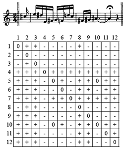
Figure 1. An excerpted phrase from Schoenberg (Op. 19, No. 4) identified by Morris (1993), and a COM-matrix after Morris (1987) produced from the excerpt
(click to enlarge)
[2.1] Within the music-theoretical literature on contour, there are generally two factors to consider in making pairwise comparisons between notes: (1) which notes to compare and (2) how to compare them. The contour adjacency series is a note-to-note model (comparing only adjacent notes) that uses ternary direction [+, 0, –]. This is the model addressed by a number of perceptual studies (e.g. Dowling and Fujitani 1971, Edworthy 1982). Morris (1987) and Marvin and Laprade (Marvin and Laprade 1987) formalize an exhaustive combinatorial model, in which every note is compared to every other note, also using ternary direction (see Figure 1).(7) The second factor—how to compare pitch height—raises the question, What is contour? Is it direction? Or is it direction and magnitude? Polansky and Bassein introduce the concept of non-ternary (n-ary) contour values, exemplified by the quintary categories: “a lot less than, less than, equal to, greater than, and a lot greater than” (1992, 277–78).(8) Similar meta-intervals (with both direction and magnitude) have been proposed for tone languages and used by the refined contour search parameter of Huron’s ThemeFinder algorithm (Huron and Sapp 1999). Though the magnitude component of refined (or n-ary) contour is generic, a case can be made for avoiding magnitude altogether in pitch height comparisons. Frequency ratio and tonal context strongly influence the perception of magnitude, but not direction. Demany, Semal, and Pressnitzer (2011) provide experimental evidence that judgment of direction (as in ternary contour) is nearly autonomic while judgment of magnitude is a higher-order cognitive process. In general, beyond pitch height comparisons, unidimensional judgment of magnitude is difficult (Donkin, Heathcote, and Brown 2015). In Marvin and Laprade (1987), contour intervals arise from multiple degrees of adjacency, not incorporating generic magnitude. Ian Quinn (1997) takes n-ary contour in the opposite (smaller) direction, with binary C+ ascent, but ternary categories can still be deduced by making pairwise comparisons in both directions (see Section 4). Because the judgment of magnitude is highly contextual, variable across cultures and between people, my position is that magnitude should be left out of pairwise contour comparisons. Choosing which notes to compare (the degrees of adjacency) is a harder decision.
[2.2] My interest lies in identifying melodic patterns intentionally developed by musicians and/or salient to attentive listeners. Where the boundary lies between what is aurally apparent (e.g. a melodic sequence) and what is beneath the surface (e.g. an Urlinie) is not known, but there is some evidence. Perceptual studies from the 1970s and 1980s(9) suggest that contour is the most prominent and memorable aspect of novel or transposed melodies outside of or prior to the establishment of a tonal paradigm. Performance of perceptual judgment tasks decreases as the length of melody increases from three to seven pitches, and rapidly erodes beyond lengths of nine pitches (Edworthy 1985, 383). Fewer empirical studies have addressed the perception of non-adjacent pairwise comparisons. A study by Quinn suggests that melodies with adjacent and non-adjacent equivalence are more likely to be categorized as similar by listeners than melodies that only share a contour adjacency series (1999, 454).(10) Edworthy’s participants struggled to retain contours of cardinality nine, so it seems reasonable to argue that eight degrees of adjacency greater, as found in a COM-matrix for a nine-pitch segment, are beyond the cognitive grasp of most listeners.
[2.3] The maximum number of degrees of adjacency for a pitch series of cardinality \(n\) is \(n-1\). For COM-matrices to be applied in analysis, phrase boundaries are needed to break up entire pitch series into segments. Using \(n-1\) degrees of adjacency for an entire piece is unwieldy, even if it is concise. Furthermore, the COM-matrix sets a high bar for formal equivalence that fails to recognize highly similar contours, such as the subject and tonal answer of Bach’s C-minor Fugue (BWV 847), as the same.(11) The alternative presented here is to commence contour analysis without any prior segmentation based on independent criteria, and lower the bar for formal equivalence by restricting degrees of adjacency to a constant window size. In analyzing a piece with a melody of 100 consecutive pitches, potentially 99 degrees of adjacency can be used. The fact that the melody starts on a higher note than it ends on may be an important and curated detail of a musical work that many listeners catch. However, what about the 3rd note and the 96th note (a comparison at the 93rd degree of adjacency)? To apply contour analysis to unsegmented music, some limits on degrees of adjacency must be imposed, even if at first they are somewhat arbitrary.
[2.4] Quinn (1999, 454) found that participants were more likely to judge contours as the same if they had equivalence beyond note-to-note comparisons. However, the effect on similarity judgments was less impressive than one might expect, and it is not known to what degree of adjacency listeners attend. Our sensitivity is likely less than \(n-1\) (the maximum for any cardinality n) in most contexts. Without prior knowledge, a listener does not know what length of segment to listen for, unless it is clearly punctuated in time. A COM-matrix for a 12-pitch segment holds 66 contour comparisons: \[ \frac{n^2 - n}{2} \] The extreme level of adjacency (\(n-1\)) may hold special prominence if heard in isolation from the rest of the piece, but it is doubtful that all degrees of adjacency hold the same sway over perception. Polansky (1996, 337) suggests a weighting for each degree of adjacency. Quinn’s study results are consistent with this (1999, 453), but he did not operationalize a test for the weighting of degrees.
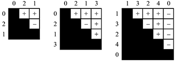
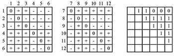
Figure 2a. COM-matrices for a segment of accumulating cardinality (the third matrix adds a new minimum)
(click to enlarge)
[2.5] The decrease in performance beyond a cardinality of nine found by Edworthy (1985, 383) bears some resemblance to Miller’s rule for mental processing of information: working memory can hold “seven plus or minus two” objects (1956). The heuristic can only be applied loosely here because the same listener may remember pitch information differently depending on context. For a listener without absolute pitch perception and acculturated to a tonal system, once a tonal context is in effect, echoic memory is likely using the same referent (tonic) for all pitches in a series. In the absence of a tonal paradigm, or before it has been established, this cannot be the case. Whether holding nine notes in terms of a tonal referent or eight directions between nine pitches in a contour adjacency series, a cardinality of nine notes is close to Miller’s upper extent of nine objects if each note corresponds to around one memory bin. The extent to which further degrees of adjacency make a contour model more or less like echoic memory of melody can only be conjectured here. Using ternary contour categories \([+, 0, -]\), a segment of cardinality nine has 15 pairwise comparisons within two degrees of adjacency (\(n\!-\!1\:+\:n\!-\!2\)) and 21 for three degrees of adjacency (\(n\!-\!1\:+\:n\!-\!2\:+\:n\!-\!3\)).(12) If each cell of a COM-matrix is an object, then Miller’s upper limit of nine memory bins is reached rather quickly (see Figure 2a). The number of unique comparisons for \(n-1\) degrees of adjacency reaches 10 at a cardinality of \(n=5\). However, it is not the pairwise comparisons that correspond to Miller’s memory bins. The contour comparisons (though ternary in the COM-matrix) are closer to bit values that encode a description of the object—in this case, the pitch.(13) Miller uses information theory to address auditory perception (pitch and loudness), in addition to other modes of perception including vision. For pitch, Miller interprets results from Pollack’s study of pitch memory (1952), wherein participants were asked to remember a collection of numbered pitches and then respond to pitch stimuli with the corresponding number. Participants tended to make identification errors when primed with collections of six or more pitches. Based on this, Pollack made a calculation of human “channel capacity” for pitch objects: a bit depth of 2.3 (1952, 748).(14) While both Pollack and Miller define it as an absolute judgment task,(15) it is more likely a judgment of relative pitch for most listeners. Participants were primed for the task in Pollack’s study by hearing a pitch collection in series from low to high, so the ordinal number of the pitch was also its relative height within the series.
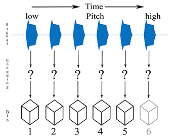
Figure 2b. Channel coding of a pitch series into working memory bins, based on Pollack (1952) and Miller (1956))
(click to enlarge)
[2.6] Let us consider the cognitive process of Pollack’s participants, however speculative. First, the primer needs to be memorized; at first, let us presume that this is done in chronological (and ascending) order. Figure 2b leaves the channel coding open, but reflects the upper limit of six pitches.(16) Many listeners would contextualize the series based on the pitch relationships therein and not recognizing absolute frequency. Out of a tonal context, recognizing super-particular ratios would be useful for trained musicians, but not for others, and such ratios were not present in the series (an equal logarithmic spacing of pitches ranging from 100 to 8000 Hz). In a tonal context, scale degrees or solmization would be quite effective, but that is not possible with this task either. A series of six pitches evenly distributed across this range is quite spread out. Each pitch would produce a distinct sensation because of the wide spacing and dispersion of corresponding sensitivity on the basilar membrane. Two pitches spread across this range are easily categorized as high and low, a distinction that perhaps can be based purely on sensation. For four pitches, we could add categories of mid-high and mid-low (categories of tone level often used in Autosegmental Phonology).
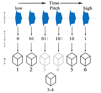
Figure 2c. Revised channel-coding model with a fusing of middle bins
(click to enlarge)
[2.7] At some cardinality, added memory bins are no longer discrete and the objects within them tend to be confused. Pollack found this effect at six pitches. However, Pollack found that inaccuracy did not tend to occur in judgments of the highest pitch stimuli, as shown in Figure 2b. Once the cardinality exceeded five, middle pitches were associated with greater error than the extremes (low and high) of the series.(17) Presumably, the bit depth of 2.3 represents a conversion of the decimal integer six to a binary integer 110 (eight integers requires a bit depth of three, four integers a bit depth of two). This would imply a loss of information at six and above. However, the loss is not at the extremes; it is in the middle. Hence, the first bit should differentiate the lowest pitch and the highest pitch, and added bits can specify relative pitch heights in between. Figure 2c revises Figure 2b to reflect an encoding of the pitches in the series based on relative pitch height and a merging of the middle bins into a single bin. In the bit encoding, the first logical represents low (0) or high (1); a second logical is added if the pitch is below (0) or above (1), the extreme represented by the first value. We could continue adding logicals as we move further and further towards the middle, but already by the third logical we have surpassed Pollack’s proposed bit depth of 2.3. In the study, response time was unrestricted, so a possible cognitive process is to compare the stimulus with echoic memory of the primer. As a participant, I would compare the stimulus to the primed low-to-high pitch series to find a match, then reconfirm the placement of that pitch in the series by comparing it to the others, e.g. “this sounds like the note that was immediately higher than the lowest note, which places it second in a series from low-to-high.” Matching the stimulus to a pitch from the primer may be an absolute frequency identification using associative memory, but assigning the stimulus a number from the series is a relative frequency comparison using syntagmatic features, and most likely does not involve magnitude (interval size) so much as direction (contour).(18)
Figure 2d. C+ matrices for a segment of accumulating cardinality (after Quinn 1997)
(click to enlarge)
[2.8] Alternatives to Miller’s magic number have been proposed, usually smaller ones. What is bewildering is how a variety of objects, whether pitch or color, correspond to the memory bins indexed by the bits. Points on a line, color, pitch, and loudness are all categorized as objects on a unidimensional continuum in Miller’s paper, but they are not uniform in terms of neural pathways or processes. This may explain some of the variation in channel capacity between the modes presented in Miller’s article. For instance, a bit depth of 3.2 is calculated for points on a line (which is right around nine objects). If channel coding has relevance to pitch perception, binary comparisons of pitch height (1 for higher, 0 for equal or lower), as suggested by Quinn (1997), are a possibility for encoding pitch syntagmatically. Quinn’s and my own reasoning for adopting binary C+ ascent \([1,0]\) over the ternary \([+, 0, -]\) model are further addressed in Section 4. For channel coding of fully combinatorial contour, as in a C+ matrix, each degree of adjacency requires a bit (see Figure 2d). A C+ matrix for three notes requires two bits, four notes require three bits, five notes four bits, and so on. Using C+ ascent with \(n-1\) degrees of adjacency is not as economical in terms of bits as the encoding shown in Figure 2c, but it is more robust (the encoding in Figure 2c is intended for a distinctly non-musical pitch series from low to high). If Pollack’s and Miller’s application of information theory has any bearing on short-term memory of contour, and if—as Quinn’s study results suggest—Polansky’s notion of “memory decay” is valid, full combinatorial contour may yield too much detail. In continuous (un-segmented) music, local degrees of adjacency beyond three may not be salient, and therefore may not be relevant to an analytical technique based on normative perception, as contour analysis is.(19)
3. Manual Segmentation
[3.1] Morris (1993) presents an analysis of the melodic foreground of a Schoenberg piano miniature (op. 19, no. 4). He introduces an algorithm that reduces phrase segments to the relationship between time and pitch extremes (the first, the last, the highest, and the lowest). Unlike the COM-matrix, the contour reduction algorithm is not sensitive to cardinality. Like the COM-matrix, it cannot be applied meaningfully until the piece is segmented. If anything, segmentation is more crucial; without it, an entire piece is reduced to a prime of (at most) four elements. Morris’s extraction of the melodic voice from the full texture of op. 19, no. 4 (which has block chords interspersed) is uncomplicated, but the segmentation into phrases deserves more exploration. The careful elaboration of the contour reduction algorithm starkly contrasts this single sentence used to describe the entire process of segmenting the piece into phrases: “Phrase boundaries conform to traditional criteria: slurs and other forms of articulation, punctuating gaps, shape, and referential affinity” (Morris 1993, 209). Two of Morris’s criteria for segmentation sound a lot like contour: “shape, and referential affinity.” His description indicates that he segmented the work by visually examining a score. So, contour was used liberally as a visual gestalt in segmenting the work, and then very methodically to reduce each segmented phrase.
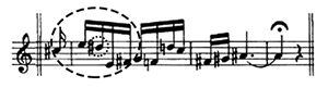
Figure 3a. Schoenberg, op. 19 no.4, segmented into phrases (from Morris 1993, 214)

(click to enlarge)
Figure 3b. Morris’s phrase 2 decomposed into two similar segments, CSIM=0.80
(click to enlarge)
[3.2] In examining Figure 3a at first glance, without detailed attention to pitch, we can see that phrase 1 and phrase 4 have similar contours, in a different range and with different durations. The variation in interval magnitude means it is not an exact transposition. Phrase 4 has two sets of recurring pitches (F4–F4 and
4. Making a CONTCOM
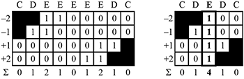
[4.1] Ian Quinn introduced the C+ Matrix in 1997 to allow an averaging of cells into fuzzy values. Quinn writes:
To find the essence of contour is tricky because there are so many ways of notating contour. Pictures, contour-pitches, and COM (comparison) matrices come immediately to mind as candidates. None of these modes of representation, however, captures the essence of contour as simply and elegantly as does one simple relation: ascent. (Quinn 1997, 248)
Figure 4a. Morris’s phrase 2 with a 4-degree window around the third pitch (the focus)
(click to enlarge)
Figure 4b. COM-matrix of phrase 2 (as in Figure 1) converted to a C+ Matrix (after Quinn 1997)
(click to enlarge)
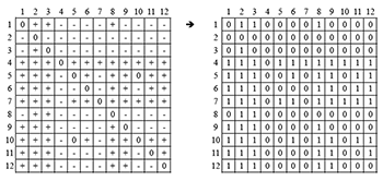
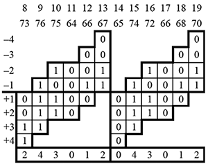
Figure 4c. Clockwise from top left: (1) C+ matrix with two degrees of adjacency above and below the main diagonal in bold, (2) the same diagonals extracted with the partial column for the third pitch (reflecting the window in Figure 4a) in bold, (3) values for the third pitch “sliced” from the C+ matrix, (4) a four-degree continuous C+ matrix (CONTCOM4) for phrase 2 (MIDI pitch values above), (5) a CONTCOM4 for all of Schoenberg, op. 19, no. 4.
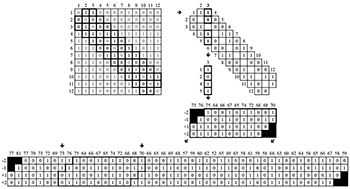
(click to enlarge)
Here, binary C+ ascent is also adopted for simplicity and elegance, but not primarily for the purpose of averaging crisp matrices into fuzzy matrices. Binary categories of 1 (ascending) or 0 (non-ascending) make techniques developed for symbolic music (MIDI data) extensible to recorded music for which categorizing note-level (or syllable- or phoneme-level) pitch segments as the same is more challenging.(20) Figures 4a–c present a new type of contour matrix intended to model contour for an entire unsegmented pitch series. A conventional COM-matrix has \(n-1\) distinct degrees of adjacency (the main diagonal in the matrix compares the event with itself). The last degree of adjacency (\(n-1\)) within a COM matrix only compares the last note to the first note (and vice versa). This contrasts the note-to-note model (e.g. Friedmann’s CAS) explored in perceptual studies (by Dowling, Edworthy, and others). Music theorists other than Friedmann have emphasized further degrees of adjacency beyond immediate neighbors, but as explained in Section 2, using all degrees of adjacency may be excessive.
[4.2] To be created, a continuous C+ matrix (CONTCOM) requires a limit on degrees of adjacency, avoiding an all-or-nothing approach to complex adjacency.(21) Beyond our perceptual framework, there are practical considerations for setting the degrees of adjacency that will be used in the CONTCOM. First, consider the minimum cardinality of segments. The total number of degrees should not exceed the minimum cardinality of interest. Then, consider the standard of equivalence for the analysis. The level of detail in a CONTCOM increases with the number of degrees of adjacency included. The lower the degrees, the lower the standard for equivalence. In the CONTCOM in Figure 4c, two degrees of pre- and post-adjacency are used for each pitch in the series, an adjacency radius of two around the focused event (the note compared to others at each index). The window size is indicated by adding a subscript to the CONTCOM label (e.g. CONTCOM4). If it is not symmetrical about the focus, orientation can also be indicated. For pitch streams of indefinite length, and to model real-time perception of pitch, a CONTCOM–2 would be appropriate, in which two degrees are extended backwards in time, as indicated by the negative. Hearing into the future is not so concrete as comparing a note to the notes before it; however, CONTCOM+2 might be useful to model expectation.
[4.3] CONTCOM is not without precedent. As noted in the introduction, Polansky (1996) uses windowing to calculate metrics in a continuous (unsegmented) signal, but there are some key differences. Polansky’s metrics (including Ordered and Unordered Combinatorial Distance) describe contour within a window, whereas the columns of CONTCOM describe a single note (or pitch segment) in relationship to other notes within a window. Any segment of CONTCOM will be composed of data from multiple windows, with windowed data for each element of the contour segment. This is a nuanced idea theoretically, but also important formally and computationally. The strongest formal connection between CONTCOM and prior contour theory is between the diagonals of a full combinatorial matrix and CONTCOM’s rows (see Figure 4c). The rows of a CONTCOM are generally a lot longer than matrix diagonals, because they may span an entire piece. Marvin and Laprade (1987) call the diagonals above the central diagonal of a COM-matrix INT1, INT2, and so on to INTn−1. INTs correspond to the rows of CONTCOM. Because binary C+ ascent is used, it is preferable to include degrees of adjacency on both sides of the focus, which could be termed INT–1, INT–2 and so on. Quinn (1997, 1999) emphasizes that C+ comparisons do not differentiate between the “0” and “−” categories of ternary comparisons, so it is necessary to use the entire C+ matrix (excluding the central diagonal) to calculate similarity (C+SIM).(22) Likewise, it is necessary to include pre- and post-adjacent comparisons to know if there is a locally repeated pitch in a CONTCOM.
5. Contour Slices, Contour Levels and Reduction
[5.1] Each column of the CONTCOM in Figure 4c is a contour slice: a collection of pairwise comparisons between a focused note and referents within a window. A radius of two degrees of adjacency around the focus forms a window of four degrees, a three-degree radius forms a window of six degrees, and so on. It is also possible to use an asymmetrical number of pre- and post-adjacent degrees. CONTCOM easily adapts to any such configuration, symmetrical or asymmetrical. Slices within each other’s window range are to some extent dependent. The +1 degree cell of a slice is the inverse comparison of the −1 degree cell of the next. Even with the partial redundancy,(23) there are six independent comparisons in two adjacent slices of a CONTCOM4. While non-adjacent degrees are useful, piling on degrees quickly becomes overly descriptive. In this demonstration of CONTCOM, an adjacency radius of two degrees (a symmetrically-oriented window of four degrees) is used to grant flexibility to pattern-match contours that do not share the same COM-matrix. With this extent of adjacency, automated analysis is fairly efficient and performs robustly.
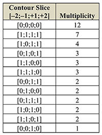
Table 5a. Multiplicity of Contour Slices (from highest to lowest)
(click to enlarge)
Table 5b. Multiplicity of Contour Levels
(click to enlarge)
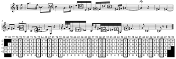
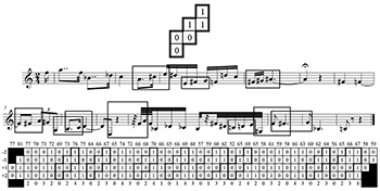
[5.2] CSEGs map pitches to contour pitches positioned low \((0)\) to high \((n-1)\) in contour space (see Marvin and Laprade 1987). With a moving window of adjacency, height in contour space is fundamentally different. Each pitch is not assigned a unique contour pitch, but a contour level that is shared by notes with different absolute pitch. Contour levels (CLs) are the sums of the contour slices. The number of levels (including 0) is the number of degrees in the window plus one. For a four-degree window, there are five levels \([0, 1, 2, 3, 4]\). Contour slices and contour levels are like the columns of a COM-matrix and contour pitches, but windowed. The windowing bears some resemblance to the Ordered and Unordered Combinatorial Distance (OCD and UCD) metrics of Polansky (1996). One use of CONTCOM that deserves further elaboration in other writings is to search or similar contour slices. There is equivalence in which every element in the slice is the same as another slice (Table 5a and Figure 5a) and similarity through the sum of ascents (the contour level, Table 5b and Figure 5b). In Schoenberg’s op. 19, no. 4, local minima \([0;0;0;0]\) have the highest frequency, followed by local maxima \([1;1;1;1]\). A species of super-minima \([0;0;1;0]\) occurs only once, and four slices (including two types of super-minima, \([1;0;0;0]\) and \([0;0;0;1]\)) do not appear at all. Slices can also be grouped by their sums (contour level), forming five genera when four degrees are used: minima (one species), super-minima (four species), mediants (six species), sub-maxima (four species), and maxima (one species). Events grouped by contour level give a different perspective on Schoenberg’s melody: there are more sub-maxima (11) and mediants (10) than maxima (7, see Table 5b). In Figure 5b, sub-maxima are boxed on the score and in bold in the CONTCOM. Slices 27 and 28 are at the same level, but sub-maximal to different maxima (these are the adjacent slices in bold outline, C4 and D4 on the score). Slice 27 (C4) is sub-maximal to 28 (D4), but 28 is sub-maximal to 30 (F4), which is not a sub-maximum at all. With a larger window of pairwise comparisons for each note, neither would be a sub-maxima. The unique properties of slices and levels are a bit confounding, but also make them a useful abstraction.
|
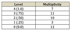
Figure 5a. The score and CONTCOM with the most common slice [0;0;0;0] boxed and in bold, and the least common slice [0;0;1;0] circled and italicized
(click to enlarge) |
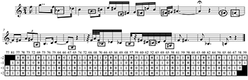
Figure 5b. The score and CONTCOM (with an added row for Contour Levels) with sub-maxima (windowed pitch height of 3 out of 4) boxed
(click to enlarge) |
6. Searching CONTCOM and the Cardinality Saturation Point
Figure 6a. Frequency for each dyad type, the piece includes no adjacent repeated pitches
(click to enlarge)
Figure 6b. Score and CONTCOM with the most common melodic triad (CSEG <012>) boxed
(click to enlarge)
[6.1] There are other useful interpretations of pitch data using CONTCOM, but my primary motivation here is finding optimal segmentations. First, I implemented a simple algorithm in MATLAB to search for the most common melodic segments of a single cardinality. The algorithm approaches the search with no information about the piece except an ordinal pitch series. Figures 6a-f are unique applications of the search algorithm to six different cardinalities starting with two and augmenting the segment size until there are diminishing returns, which for this piece is cardinality seven. Greater sizes could easily be searched for as well, but beyond a certain cardinality, there is no recursion at all.
[6.2] The algorithm excludes cells that compare the focus to referents outside of the segment, so the dyad does not take advantage of the non-adjacent degrees included in CONTCOM4 (see Figure 6a). All dyads in the Schoenberg miniature are either ascents or descents; there are no horizontal dyads. In Figure 6b, the most common melodic triad is shown as the search algorithm sees it. In contrast to the contour slice, this jagged excerpt of the CONTCOM4 gives complete contour information (as in a C+ matrix) about the relationships between three adjacent elements, but nothing about their relationship to outside pitches. Dyads and triads were identified as basic building blocks of melodic contour by Seeger (1960) and Kolinski (1965). The sub-segmental nature of these lower cardinalities is reflected in the decomposition of CSEGs into CSUBSEGs by Marvin and Laprade (1987). Figure 6a and 6b demonstrate the over-segmentation that occurs when the algorithm searches for cardinalities two and three.
|
Figure 6c. CONTCOM with the most common melodic tetrad in bold
(click to enlarge) Figure 6e. Score and CONTCOM with the most common melodic hexad boxed
(click to enlarge) |
Figure 6d. Score and CONTCOM with the most common melodic pentad boxed
(click to enlarge) Figure 6f. Score and CONTCOM with the most common melodic heptad boxed
(click to enlarge) |
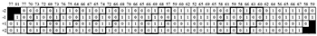
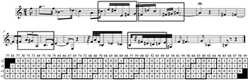
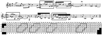
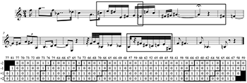
Table 6a. The cardinality saturation point for the Schoenberg miniature is 9
(click to enlarge)
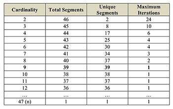
[6.3] As the cardinality increases, the amount of recursion of a single segment decreases (see Table 6a). For cardinality four, the most common contour segment has six instances, as compared with 10 for triads. At four, contours more characteristic of the piece begin to appear. At cardinality six, a meaningful analysis emerges. The high-frequency hexad has the same starting points as the high-frequency pentad, but neatly closes the gap between the first and second occurrences, filling out Morris’s phrase 2. A constraint on the search algorithm could be added to exclude contour segments that span rests. As Tenney and Polansky note, temporal separation has a segregative effect on a monophonic succession of elements (1980, 208). If such a constraint were added, all the identified hexads would fall within Morris’ phrase boundaries (Figure 3a). Cardinality six provides the optimal segmentation using a single pattern. Extending the search algorithm to cardinality seven reduces the number of items returned by the most common segment, so there is less coverage (\(7\!\times\!3 < 6\!\times\!4\)), and two of Morris’s phrase boundaries are crossed.
[6.4] A trend emerges from increasing the cardinality of the search algorithm. In this piece and all others I have studied, a point is reached beyond which every segment is unique and there is no recursion: the cardinality saturation point. In the Schoenberg miniature, the cardinality saturation point is nine. At this and greater segment lengths, the total number of segments equals the number of unique segments, and both decrease until the cardinality of the entire series is reached (see Table 6a). Beyond the saturation point, there is no recursion. In the lower cardinalities the number of unique segments is at or near the possible number of permutations. For a piece with considerable contour recursion, such as this Schoenberg miniature, the number of unique segments does not keep pace with the number of possible permutations as cardinality increases.
7. Segmentation Algorithm
Figure 7a. A ground truth for the contour search algorithm, with two recursive segments (one circled and one boxed)
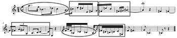
(click to enlarge)
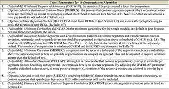
Table 7a. Input Parameters for the Segmentation Algorithm
(click to enlarge)
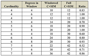
Table 7b. Number of cells for windowed C+SIM and full C+SIM (n-1) for various cardinalities and window sizes
(click to enlarge)
Figure 7b. RCS reduction process for a C4 to C5 chromatic scale

(click to enlarge)
Figure 7c. RCS reduction process for a C-major arpeggio

(click to enlarge)
Figure 7d. RCS reduction process for repeated pitches

(click to enlarge)
Figure 7e. Schoenberg, op. 19, no.4 includes two redundant contour slices and no consecutive repeated pitches
(click to enlarge)
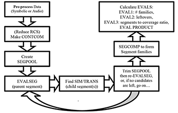
[7.1] Based in part on Morris’s phrase boundaries, a ground truth for automatic segmentation appears in Figure 7a. This serves as an empirical standard that, if successful, the algorithm will replicate without any information specific to the piece except for the pitch values, onsets and offsets. Over 83% of the pitch series (39 out of 47 events) can be accounted for with two model segments. The circle motive is a heptad and the boxed motive is in most cases a hexad. The third appearance of the boxed motive is extended into a heptad by a redundant contour slice (see [7.2]); the fourth appearance is a similar contour in retrograde. Because the ground truth uses multiple cardinalities, the segmentation algorithm must search and pick segments of multiple cardinalities to succeed. The constraints and methods in Table 7a are also added to improve the algorithm. As input parameters, they can be turned “on” or “off” or adjusted to be appropriate to the musical object being analyzed. The parameters are restricted to pitch information, with the exception of number 8, SEEGAP. Of the parameters, 1–3 effect creating and pre-processing the CONTCOM, 4 is a constraint on cardinality, 5 augments the search algorithm by implementing a secondary search for transformations of recursive segments within the segment pool (SEGPOOL), and 6–9 filter or evaluate candidates in the SEGPOOL.
[7.2] Of these parameters, one in particular deserves elaboration: REDRCS, the reduction of redundant contour slices. It is a novel solution to the cardinality sensitivity problem made possible through the formalization of contour slices (a similar reduction can be applied to contour levels). Through the reduction, melodic segments of different lengths may form equivalent contour segments. Unlike other methods, reduction is applied to the entire series before segments are identified. There are no cardinal primes because in contour-level space all maxima and minima are equal (level n and level 0 respectively). Slices for two or more consecutive unaccented notes are reduced to one, specifically passing or repeated tones and not notes at a change of direction, which Thomassen calls pivots (1982). Redundant contour slices (RCSs) are defined here as consecutive columns in CONTCOM that hold the same adjacent relationships (\(\pm 1\) degree) as the previous column. In its application to ascending or descending motions, the reduction mirrors the fusing of middle memory bins in Figure 2c. For example, an ascending chromatic scale from C4 (MIDI pitch 60) to C5 (MIDI pitch 72) is reduced to the first slice, the last slice, and one intermediate slice (see Figure 7b). Likewise, an ascending C-major arpeggio is reduced to three slices (see Figure 7c). The reduction is the same in terms of adjacent degrees (as pictured). However, cells for non-adjacent comparisons will need to be recalculated based on a new mean pitch. There is no information for the relationship of the first pitch to a prior pitch or the final pitch to later pitches, making them distinct from the intermediate notes in that they are under-contextualized. As Pollack (1952) found, the first pitch and the last pitch of a finite pitch series have special prominence. In addition to initials and finals, local minima and maxima are never eliminated through this process, and although it has similarities to Morris’s algorithm, it is considerably less drastic than reduction to a prime. All pivots and at least one medial event between pivots (if there is one) are kept. REDRCS may reduce some slices for repeated pitches, but it does not remove them all. Figure 7d shows the reduction for a segment of the same length as the chromatic scale in Figure 7b, but with many repeated pitches in the center instead of stepwise ascent. This produces a longer reduced contour because the first event at 66 (
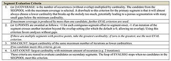
Table 7c. Segment evaluation criteria
(click to enlarge)
Figure 7f. Workflow for the segmentation algorithm
(click to enlarge)
[7.3] After preparing the CONTCOM (with or without reduction), the search module returns indices in a segment pool (SEGPOOL) for occurrences of each unique segment of CONTCOM within the constraints of the input parameters. For each cardinality, the most common segment is presented to the segment evaluation module (EVALSEG) as a candidate to be the primary segment. Multiple ranked evaluation criteria are used to select from the full range of cardinalities in the SEGPOOL (see Table 7c). An input parameter, COVRPNTS, determines the first criterion for evaluating candidates in the SEGPOOL. Points is intended for tightly-constructed music with close recursion (such as this composition by Schoenberg), and coverage is intended for music with frequent paradigmatic cadences, and all else. Selecting the primary segment (the first parent segment) is the most crucial step. After this point, only segments that fit into the relief left by the primary segment are used.
[7.4] The workflow in Figure 7f produces a single analysis. This process may be run repeatedly, varying a single parameter at a time within a range, before a final evaluation of multiple analyses. In the SEGCOMP phase, if the indices of a superior parent segment's child segments (similar and transformed iterations) correspond with the indices of an inferior parent segment, the resulting analysis for one set of parameters may be reduced before it enters the final evaluation. A key metric for ranking analyses is the number of recursive segments used (optimum is 1). So, any reduction improves the performance of an analysis in the final evaluation. Reduction occurs when the indices of the child segments of a superior parent segment are contained by (or contain) the indices of an inferior parent segment. The inferior parent along with its children (if any) join the family of the superior segment. Even if adopted segments are not the same cardinality as the parent segment, they are still accepted. Like the reduction of redundant slices, but through a different means (that can be compounded with REDRCS), this allows for the possibility of recognizing contours of different cardinalities as related.
8. Discussion of Analyses and Comparison to Ground Truth
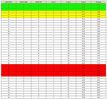
[8.1] All of the candidate analyses are ranked in a final evaluation metric, using one or more of the following criteria:
- EVAL1: Number of contour segment families;
- EVAL2: Number of pitches left out of the segmentation;
- EVAL3: Total number of segments divided by the number of leftover pitches.
Table 8a. Input parameters and evaluation of resulting analyses, ranked lowest to highest in terms of evaluation product (last column)
(click to enlarge)
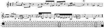
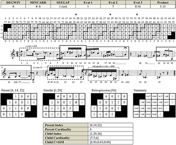
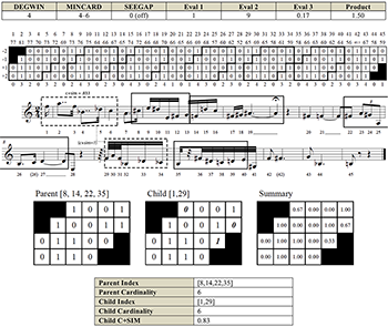
Figure 8a. Analysis 1 is highest-ranked by EVAL Product; SEEGAP is turned on (locations indicated on CONTCOM by arrows)
(click to enlarge)
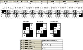
Figure 8b. Analysis 2, which is similar to Analysis 1 but with SEEPGAP turned off, allowing segments to span rests (as from event 35 to 36)
(click to enlarge)
Figure 8c. Analysis 3 is over-segmented because the minimum cardinality is too low
(click to enlarge)
For all criteria, lower values are preferred. The last criterion gives preference to larger cardinalities. Any single criterion can be used, or it can be multiplied, creating an evaluation product that is ranked higher if it is of a lower value. Table 8a is a ranked list of analyses with EVAL products less than 5. Analyses corresponding to the three boxed portions of the table are visualized in Figures 8a (Analysis 1), 8b (Analysis 2), and 8c (Analysis 3). The same analysis may be returned by similar input parameters. Analysis 1 is closest to Morris’s segmentation. Analysis 2 allows segments to cross time gaps (rests). Analysis 3 is included to illustrate over-segmentation resulting from a minimum cardinality of less than 4. For each analysis: (1) the input parameters and output evaluation criteria values are listed; (2) the CONTCOM4 is shown for the entire piece (Analyses 1 and 2 also show the score); (3) a table of the segment indices is provided; (4) the model for each segment is shown and labeled according to its rank; and (5) if there is more than one segment in a family, a weighted fuzzy summary is calculated based on the model segments and number of iterations for each model. All C+SIM values are restricted to the windowed degrees of adjacency. If the child segment(s) is larger than the parent, these additional cells are shaded gray. The fuzzy values follow Quinn (1997), with the number of iterations for each segment in the family used as a weighting in the calculation. A fuzzy matrix is just one way to summarize similarity between related segments produced by the algorithm, whether iterations of the same model or within the same family. Once one has segments, there are many, many ways to calculate degrees of similarity between them. Options for working with different cardinalities include Morris’s contour reduction algorithm (1993), Huron’s simil command in the Humdrum Toolkit (1994) and gross shapes (1996), Polansky’s Combinatorial or Linear Direction metrics (1996), phase spectra from Fourier analysis (Schmuckler 2010), and various statistical methods.
[8.2] Analyses 1 and 2 are the highest-ranking analyses by evaluation product. Rows 1–3 of Table 8a correspond to Analysis 1 (Figure 8a) and rows 4–6 to Analysis 2 (Figure 8b). Keeping the window size constant and varying the minimum cardinality (MINCARD) from four to six produced the same analysis. The difference between Analyses 1 and 2 in terms of input parameters is the setting for SEEGAP: Analysis 1 has it “on” and Analysis 2 has it “off.” “Punctuations” were part of Morris’s manual segmentation. Excluding segments that cross gaps from the SEGPOOL produces an analysis identical to the ground truth. Analysis 3 is the highest-ranking among the analyses produced with the minimum cardinality set below four. Setting a minimum cardinality of four returns segments that are characteristic of the piece, at cardinalities of six and seven, instead of over-segmenting the piece with triads that are the basic building blocks of all melodic contour (see Seeger 1960, Kolinski 1965). Using a minimum cardinality (MINCARD) of four may be a good general practice for segmentation based on contour recursion.
[8.3] Analysis 1 (Figure 8a) demonstrates that Morris’ segmentation can largely be recreated with an automated process of searching for and evaluating contour recursion. There are two exceptions: (1) leftover pitches not included in the recursive segment collection, and (2) the combination of recursive segments into a single segment, as in Morris’s phrase 2. Exception 1 can be overcome without durational information, but exception 2 cannot. In a post-segmentation module, leftover pitches could be joined to a recursive segment by adding a conditional statement: if there are leftover pitches in clusters of less than the minimum cardinality, they should be joined with the closest segment not separated by an offset-to-onset gap (rest). Any larger cluster should form a non-recursive segment of its own. This produces Morris’s phrase 3 and phrase 5. Regarding exception 2, Morris’s identification of phrase 2 seems to be based on uniformity in duration (a string of sixteenth notes), perhaps a form of “referential affinity.” Because the segmentation algorithm works with only pitch and not durational information, it does not see the larger rhythmic grouping observed by Morris. The fusion of these segments into one phrase cannot be accomplished without considering duration.
9. Recursive Segment Models (CLSEGs)
Figure 9a. Reduction of repeated pitches (DELREP) and incomplete slices
(click to enlarge)
[9.1] CONTCOM is very robust for computation, but less than ideal for visualization. In classic contour theory (e.g. Morris 1987, Marvin and Laprade 1987), the CSEG class is useful for nominalizing a contour matrix into a visually and verbally digestible format, e.g. \(< 0\, 2\, 1 >\) : “zero-two-one.” In this modified contour space, contour pitches have been replaced with contour levels. By extension, the analog to CSEGs are CLSEGs. For the Schoenberg piece, the highest-ranked analysis used CONTCOM4, so any CLSEG produced from it will be a CLSEG4, following the subscript convention for the CONTCOM indicating the window size used. In this modified contour space, every pitch is no longer distinct. A recurring pitch will have a different contour level, not some of the time, but almost always. Contour slices of all the same binary value (0s or 1s) mean the event in focus is an extreme within the window around it, but the next local minima or maxima is not likely to be at the same absolute pitch height. A conceptually challenging zero-value is produced by the first example in Figure 9a. An event that is equal to everything within its window is a local minimum. The contour level of 0 for the fifth note, though somewhat counter-intuitive, reflects a true statement: it is at the lowest pitch within a four-degree window around it. In contour-level space, repeated pitches lose and gain height as they move away or towards pitch variance. The loss or gain of windowed pitch height by repeated pitches is not necessarily a fault of CONTCOM. To the extent that this phenomenon is a detriment or benefit to the analysis of contour in music with repeated pitches (of which the Schoenberg piece is not an instance) will be explored in further research; however, it can be avoided fairly easily by collapsing all consecutive repeated pitches to a single event, as on the right side of Figure 9a. There is precedent for the elimination of repeated pitches in contour analysis by ethnomusicologists and music theorists (Polansky 1996, 261). However, this produces an anomaly that is an issue for music without consecutive pitch repetition, such as this Schoenberg piece. In the right-side example of Figure 9a, pitches a step apart (D4 and E4) map to levels 1 and 4. The wide gap has nothing to do with reducing repeated pitches and everything to do with time-extreme events, which are under-contextualized in comparison with the interior contour slices of a CONTCOM. A pitch at the beginning or ending of a musical work is phenomenologically different than a pitch in the interior of the work. CONTCOM neither assumes a genesis of pitch or absolute finality. The initial and final pitches may have more context, but that context is unknown to the CONTCOM. This does not pose any problem for the search algorithm, but it is a problem for the summation of slices into levels when some slices are incomplete. The maximum level of incomplete slices is less than the complete slices.
Figure 9b. Morris’ phrase 2, window allowed to change degree-orientation
(click to enlarge)
Figure 9c. Recursive segments from Schoenberg op.19 no. 4, with contour levels mapped to staff
(click to enlarge)
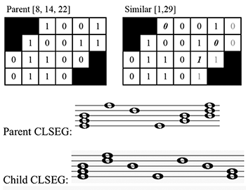
[9.2] There are three ways to handle this problem when making a CLSEG. The first is to include cells for comparisons outside of the segment, if it is not at the beginning or ending of the piece. However, that will not describe all iterations of a recursive segment. The second is to allow the orientation of a window to shift to include more degrees in one direction or the other. This works for other pieces I have studied, such as the subject of Bach’s C-minor Fugue (BWV 847), but in this case, it does not (see Figure 9b). The third option is to include a range of possible values for incomplete contour slices. For the Schoenberg piece, the last option is ideal for modeling recursive segments. In Figure 9c, the parent segment of Analysis 1 yields a CLSEG4 of \(< 0\text{-}2, 4, 3, 0, 1\text{-}2, 3\text{-}4 >\) and the child segment yields \(< 0\text{-}2, 3\text{-}4, 2, 0, 3, 2, 0\text{-}1 >\), with the dash representing a range of possible contour-level values. While the contour level for slices with complete context for the adjacency radius can be calculated through a simple summing of the column, when there is incomplete context this is not the case. An interesting case of this is in the parent segment. It appears that the second slice could be level 3 or level 4 with more context, but if we consider the +1 comparison value (to the next event), it is above it and only level 4 is an option, which in turn means the maximum possible contour level for an event immediately prior to the segment is 3. There can be multiple local minima (or other levels), but there can be only one local maximum within a radius of each other (half the window size if it is symmetrical). This creates a bit of a paradox, because a pitch prior to the segment could potentially be equal to or higher than the second event, which would create the inverse of the repeated pitch anomaly: adjacent pitches of different height with the same contour level. Once again, this is not seen as an invalidation of the model, but an interesting side effect of a new abstraction of pitch space. What it reveals to me is that although the segment is extracted from the CONTCOM4 with outside context excluded, the outside context still has a phantom presence. The model for the parent segment excludes the possibility of level 3 for event 2. Although the possibility exists within the matrix formation for consecutive events with different pitches to have the same contour level, it does not happen in the actual analysis of the piece. It is only a possibility in the model of the recursive segment and may be constrained from surfacing in the music. To some extent, each segment model dictates surrounding events, or the environments in which it is realized. This extends to recursive behavior. The parent segment is more generative and less restricted in its realizations than the child segment. This can be attributed to a specific characteristic: the beginning CL range does not enclose the ending CL range, as it does in the child segment. If iterations of the child segment were to be arranged consecutively (which they are not in this piece), selection from of a level from the range of options for the ending of the first iteration would influence the level of the beginning of the second iteration, or vice versa. For consecutive iterations of the parent segment, the realized initial or final contour level for one iteration does not restrict adjacent realizations.
Figure 9d. A mapping from the pitches of a parent segment iteration (starting at index 8) to the CSEG class (center), and finally to the C+SEGr (right)
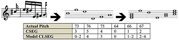
(click to enlarge)
[9.3] Each realization of an underlying contour may have a unique relationship to the model CLSEG. The easier path to consider is a mapping from the actual pitches to the model, in which information is reduced. In Figure 9d, a segment from the score is mapped to conventional contour space (CSEG class \(<354012>\)) and then on to contour level (CL) space. As a further abstraction, the CLSEG can be calculated directly from the pitch series or the CSEG class. It matters not. The mapping from the symbolic data to the CSEG class is lossless in terms of the information needed to create a CLSEG model. The CSEG can be an intermediary step in the mapping, or bypassed. Defining the inverse mapping from the model to the actual pitches is more complicated because it requires the gaining of information: specification from a very general model to what we actually see in the music. The information gained is largely influenced by external musical constraints. For many instruments there are physical constraints, or a composer or improviser may be working with a specific pitch set or scale. There is infinite potential for realization of each CLSEG, as there are for CSEGs. This infinity is tangibly, but perhaps not truly, augmented by realizations that augment the cardinality. Is it possible to narrow this down to likely and unlikely realizations? A heuristic for this may be Prince and Smolensky’s Optimality Theory (2004),(24) a phonological method inspired in part by Lerdahl and Jackendoff’s GTTM (1983), which in turn took cues from generative linguistics. In its nascent form, optimality theory evaluates candidate words by ranking constraints that explain why one word surfaces in the lexicon instead of other conceivable or improbable words. Generally, constraints that exclude improbable words are easier to come by. When using OT, one does not know all of the inputs. They are hypothetical save for the one that will be the successful candidate. More than the single output, the formulation and ranking of constraints is of interest here. Any CLSEG can generate as many inputs to be evaluated by a constraint ranking as one can imagine. For there to be recursion, multiple realizations of the CLSEG must succeed in the evaluation. Not to conflate music and language or words and melodic segments, but a ranking of constraints on outputs may be very useful for mapping a segment in contour space to pitch space. Any constraints would reflect important traits of style and idiom, such as whether it is diatonic or non-diatonic music, and what voice range or instruments will perform the music. Exploring the inverse mapping from models to realizations is not a simple task, but may be very fruitful.
10. Conclusion
[10.1] Through the application to a single piece of music, it is possible that I have “over-fit” the method. However, Schoenberg’s compositional idiom is so methodical and influential that the method, as presented here, should be extensible to much art music of the twentieth century at the very least. While other music may pose unique challenges to the method, the intention behind including variable parameters is so that it can also be applied to a wide assortment of monophony and monophonic extractions from other textures. Schoenberg’s music is a good testing ground because it is so consciously crafted, but it is not unique in its recursive nature. The following challenges to broader application were accommodated in the initial formulation:
- This analysis privileged candidate segments with close recursion, awarding “points” for iterations that are adjacent without overlapping. For tonal music, an alternative criterion of “coverage” is provided for segment evaluation (see Table 7c).
- This analysis is of a pitch series of finite length. The ability to handle pitch streams of indefinite length is necessary for online processing or modeling real-time listening. Both of these applications make an adjacency radius around the focus (and comparisons to the past and future) less appropriate. A window of only pre-adjacent degrees can be used.
- Analysis of monophonic recordings poses a unique challenge that cannot be addressed sufficiently here: segmentation of an audio signal into an ordinal pitch series. Proprietary software exists that can accomplish this task, notably Melodyne, but it is preferable to have more user control over the calculation of a pitch from a fundamental frequency analysis, as well as some signal-sensitive parameters. In further research, manual pitch segmentation will be compared with automated approaches, in hopes of creating a fully automated process from raw audio to pitch series to melodic segments.
Additionally, detailed exploration and discussion of the contour slice, contour level and the recursive segment model (CLSEG) is needed.
[10.2] The processing load for the current algorithm is heavy. To approximate the ability of a trained music analyst to recognize what Morris terms “shape and referential affinity” is quite taxing for a computer. This load could be reduced somewhat by knowing more about human perception of contour, which could in turn reduce the number of different analyses attempted with varying input parameters. What is lacking is a perceptual basis for how many degrees of adjacency are salient. One way to get more information is to conduct more behavioral studies. One could look for trends in similarity ratings for melodies that have the same contour at two but not three degrees of adjacency, three but not four degrees, four but not five degrees, and so on. This is similar to methods used by Dowling (Dowling and Fujitani 1971) and Edworthy (1982) to study simple-adjacency, and by Quinn for complex-adjacency (1999). Another method, similar to Edworthy (1985), is to ask listeners to make non-adjacent pairwise comparisons and look for a drop-off in accuracy or response time. Experiments to reveal perceptual or cognitive limits of non-adjacent contour comparisons would provide greater explanatory adequacy for using a specific window size. Experiments by Schmuckler (2010) compare contours of the same length of time instead of cardinality.(25) No doubt, the duration of notes and metric placement affects salience. However, I prefer to consider them as parallel streams that are to some extent independent, like having a CSEG and a DSEG for the same segment (Marvin 1991). This reflects the role of contour in Schoenberg’s op. 19, no. 4, as well as the tone-level systems of Niger-Congo languages that inspired this revision of contour theory.(26) Further behavioral research would lead to only modest improvement in the method presented in this article, because it is already clear from this and other analyses that a fairly small window of two to six degrees is most effective. My speculation is that this is similar to the human capacity for non-adjacency, which is without doubt variable.
[10.3] The extent to which non-adjacent comparisons are perceptually salient is not known, but simple-adjacency has been thoroughly researched. A happy medium between simple-adjacency and exhaustive comparison reflects our knowledge of pitch perception and is productive analytically. Through automation, this analytical approach has potential for application to large corpora, and to the use of machine learning to improve efficiency. Constraining the range of input parameter values to only the most productive would be much less costly in terms of processing than producing many analyses and ranking them. However, the flexibility of the window size and other parameters make this method extensible. The re-ranking of SEGPOOL evaluation criteria (see Table 7c) is only one way to adapt this method to other signals. Schoenberg’s op. 19, no. 4 was selected as an object of analysis because of its brevity and to make a connection to prior work, specifically Morris 1993. This does not reflect limitations on its use or efficacy. Unlike the COM-matrix, intended for music such as Schoenberg’s, CONTCOM and the segmentation algorithm are designed for and have been applied to diverse musical spaces, including Bach’s Well-Tempered Clavier, trumpet solos by Dizzy Gillespie, Ìgbò choral music, and Yorùbá praise poetry.(27) This modified toolbox for contour analysis maintains applicability to past analyses and holds promise for analyzing a wide range of monophonic sound and symbol.
Aaron Carter-Ényì
Ohio State University
School of Music
Columbus, OH 43210
carterenyi@gmail.com
Works Cited
Adams, Charles R. 1976. “Melodic Contour Typology.” Ethnomusicology 20 (2): 179–215.
Beard, R. Daniel. 2003. Contour Modeling by Multiple Linear Regression of the Nineteen Piano Sonatas by Mozart. PhD diss., Florida State University.
Bidelman, Gavin M., and W. L. Chung. 2015. “Tone-Language Speakers Show Hemispheric Specialization and Differential Cortical Processing of Contour and Interval Cues for Pitch.” Neuroscience 305: 384–92.
—————. 2010. “Cross-Domain Effects of Music and Language Experience on the Representation of Pitch in the Human Auditory Brainstem.” Journal of Cognitive Neuroscience 23 (2): 425–34.
Bor, Mustafa. 2009. Contour Reduction Algorithms: A Theory of Pitch and Duration Hierarchies for Post-Tonal Music. PhD diss., University of British Columbia.
Carter-Ényì, Aaron. 2016. Contour Levels: An Abstraction of Pitch Space based on African Tone Systems. PhD diss., Ohio State University.
de Cheveigne, Alain. “Pitch Perception Models.” In Pitch: Neural Coding and Perception, edited by C. J. Plack, Andrew J. Oxenham, R. R. Fay and N. A. Popper, 169-233. New York: Springer, 2005.
Demany, Laurent, Catherine Semal, and Daniel Pressnitzer. 2011. “Implicit Versus Explicit Frequency Comparisons: Two Mechanisms of Auditory Change Detection.” Journal of Experimental Psychology: Human Perception and Performance 37 (2): 597.
Donkin, Chris, Babette Rae Andrew Heathcote, and Scott D Brown. 2015. “Why Is Accurately Labelling Simple Magnitudes So Hard? A Past, Present and Future Look at Simple Perceptual Judgment.” In The Oxford Handbook of Computational and Mathematical Psychology, edited by Jerome R. Busemeyer, Zheng Wang, James T. Townsend and Ami Eidels, 121–52. Oxford University Press.
Dowling, W. Jay, and Diane S. Fujitani. 1971. “Contour, Interval, and Pitch Recognition in Memory for Melodies.” Journal of the Acoustical Society of America 49 (2B): 524–31.
Dowling, W. Jay. 1978. “Scale and Contour: Two Components of a Theory of Memory for Melodies.” Psychological review 85 (4): 341–54.
Edworthy, Judy. 1982. “Pitch and Contour in Music Processing.” Psychomusicology: Music, Mind & Brain 2 (1): 44–46.
—————. 1985. “Interval and Contour in Melody Processing.” Music Perception 2 (3): 375–88.
Eerola, Tuomas, Tommi Himberg, Petri Toiviainen, and Jukka Louhivuori. 2006. “Perceived Complexity of Western and African Folk Melodies by Western and African Listeners.” Psychology of Music 34 (3): 337–71.
Friedmann, Michael L. 1985. “A Methodology for the Discussion of Contour: Its Application to Schoenberg's Music.” Journal of Music Theory 29 (2): 223–48.
Huron, David. 1994. The Humdrum Toolkit: Reference Manual. Center for Computer Assisted Research in the Humanities.
—————. 1996. “The Melodic Arch in Western Folksongs.” Computing in Musicology 10: 3–23.
—————. 2002. “Music Information Processing Using the Humdrum Toolkit: Concepts, Examples, and Lessons.” Computer Music Journal 26 (2): 11–26.
Huron, David, and Matthew Royal. 1996. “What Is Melodic Accent? Converging Evidence from Musical Practice.” Music Perception 13 (4): 489–516.
Huron, David, and Craig Sapp. 1999. “Themefinder.” CCARH (Stanford), CSML (OSU): http://www.themefinder.org/.
Kolinski, Mieczyslaw. 1965. “The Structure of Melodic Movement: A New Method of Analysis: Revised Version.” Studies in ethnomusicology 2: 95–120.
Lartillot, Olivier. 2004. “A Musical Pattern Discovery System Founded on a Modeling of Listening Strategies.” Computer Music Journal 28 (3): 53–67.
Lerdahl, Fred, and Ray Jackendoff. 1983. A Generative Theory of Tonal Music: MIT Press.
Marvin, Elizabeth West. 1991. “The Perception of Rhythm in Non-Tonal Music: Rhythmic Contours in the Music of Edgard Varese.” Music Theory Spectrum 13 (1): 61–78.
Marvin, Elizabeth W., and Paul A. Laprade. 1987. “Relating Musical Contours: Extensions of a Theory for Contour.” Journal of Music Theory 31 (2): 225–67.
Massaro, Dominic W., Howard J. Kallman, and Janet L. Kelly. 1980. “The Role of Tone Height, Melodic Contour, and Tone Chroma in Melody Recognition.” Journal of Experimental Psychology: Human Learning and Memory 6 (1): 77–90.
Matthews, William J., and Neil Stewart. 2009. “The Effect of Interstimulus Interval on Sequential Effects in Absolute Identification.” The Quarterly Journal of Experimental Psychology 62 (10): 2014–29.
Miller, George A. 1956. “The Magical Number Seven, Plus or Minus Two: Some Limits on Our Capacity for Processing Information.” Psychological Review 63 (2): 81.
Morris, Robert D. 1987. Composition with Pitch-Classes: A Theory of Compositional Design. Yale University Press.
—————. 1993. “New Directions in the Theory and Analysis of Musical Contour.” Music Theory Spectrum 15 (2): 205–28.
Ohriner, Mitchell S. 2012. “Grouping Hierarchy and Trajectories of Pacing in Performances of Chopin’s Mazurkas.” Music Theory Online 18 (1).
Polansky, Larry. 1996. “Morphological Metrics.” Journal of New Music Research 25 (4): 289–368.
Polansky, Larry, and Richard Bassein. 1992. “Possible and Impossible Melody: Some Formal Aspects of Contour.” Journal of Music Theory 36 (2): 259–84.
Pollack, Irwin. 1952. “The Information of Elementary Auditory Displays.” The Journal of the Acoustical Society of America 24 (6): 745–49.
Prince, Alan, and Paul Smolensky. 2004. Optimality Theory: Constraint Interaction in Generative Grammar. Blackwell Publishing.
Quinn, Ian. 1997. “Fuzzy Extensions to the Theory of Contour.” Music Theory Spectrum 19 (2): 232–63.
—————. 1999. “The Combinatorial Model of Pitch Contour.” Music Perception 16 (4): 439–56.
Schmuckler, Mark A. 1999. “Testing Models of Melodic Contour Similarity.” Music Perception 16 (3): 295–326.
—————. 2010. “Melodic Contour Similarity Using Folk Melodies.” Music Perception 28 (2): 169–94.
Schultz, Robert D. 2009. “A Diachronic-Transformational Theory of Musical Contour Relations.” PhD diss., University of Washington.
Seeger, Charles. 1960. “On the Moods of a Music-Logic.” Journal of the American Musicological Society 13 (1/3): 224–61.
Sekula, Kate. 2014. “Utilizing Computer Programming to Analyze Post-Tonal Music: A Segmentation and Contour Analysis of Twentieth-Century Music for Solo Flute.” PhD diss., University of Connecticut.
Tenney, James, and Larry Polansky. 1980. “Temporal Gestalt Perception in Music.” Journal of Music Theory 24 (2): 205–41.
Thomassen, Joseph M. 1982. “Melodic Accent: Experiments and a Tentative Model.” The Journal of the Acoustical Society of America 71 (6): 1596–1605.
Footnotes
1. See Seeger 1960, Kolinski 1965, and Adams 1976.
Return to text
2. Some relevant sources from the music cognition and perception and the speech and hearing science literature include Dowling and Fujitani 1971; Dowling 1978; Massaro, Kallman, and Kelly 1980; Edworthy 1982, 1985; Quinn 1999; Schmuckler 1999; Eerola et al. 2006; Bidelman et al. 2010, 2015; and Demany, Semal, and Pressnitzer 2011.
Return to text
3. See Morris 1987.
Return to text
4. See Friedmann 1985, Marvin and Laprade 1987, Polansky and Bassein 1992, Marvin 1991, Morris 1993, Polansky 1996, Quinn 1997, Beard 2003, Schultz 2009, and Bor 2009.
Return to text
5. See Huron 1994, Lartillot 2004, and Schmuckler 2010.
Return to text
6. The nine three-point gross shapes are: ascending, descending, concave, convex, horizontal-ascending, horizontal-descending, ascending-horizontal, descending-horizontal, horizontal (Huron 1996, 9).
Return to text
7. For detailed discussion of both models see Quinn 1999.
Return to text
8. Polansky 1996 keeps direction and magnitude metrics distinct.
Return to text
9. Dowling and Fujitani 1971; Dowling 1978; Massaro, Kallman, and Kelly 1980; Edworthy 1982, 1985.
Return to text
10. A COM-matrix models complex adjacency because it involves both adjacent and non-adjacent comparisons.
Return to text
11. In an application of the segmentation algorithm to Bach’s C-minor Fugue (BWV 847), it was found that the subject and its answers are only equivalent up to 10 degrees of adjacency (adjacency radius of 5). The cardinality is 20, but all possible degrees of adjacency (19) are not relevant to determining that the subject and its answers have highly similar, even equivalent, contours. Findings on contour recursion in tonal music (including imitative polyphony and jazz improvisation) are addressed in my dissertation (Carter-Ényì 2016) and will be published in separate articles.
Return to text
12. This can be generalized as \(\Sigma(n-1 \ldots n\mathrm{-degrees})\). . . n-degrees).
Return to text
13. Both Miller 1956 and Pollack 1952 use the term tone instead of pitch.
Return to text
14. A bit depth of 2 would yield four objects and 3 would yield nine objects. Bit depth is converted to unique values by taking 2 to the power of the bit depth (e.g. \(2^x\), where \(x\) is the bit depth).
Return to text
15. In current psychology literature, this is referred to as absolute identification.
Return to text
16. Here channel coding refers to the categorization of perceived pitch in echoic memory, and bypasses the rather complex question of how a physical signal is converted to a mental impulse. See de Cheveigne 2005 for models of pitch perception from Helmholtz to more recent scholarship. Clearly, the bit depth of 2 to 3 calculated by Pollack (and reiterated by Miller) is not intended to encapsulate the complexity of pitch perception, but simply the information necessary to differentiate like sounds that differ only in terms of pitch height.
Return to text
17. Another possible cause for error in the absolute identification task is the number of stimuli between the prime and current stimulus. Recent studies (Matthews and Stewart 2009; Donkin, Heathcote, and Brown 2015) have explored sequential effects.
Return to text
18. Though not in reference to Pollack’s study or a discussion of non-adjacent comparisons, Lartillot (2004, 58–60) provides a similar account of listening strategies.
Return to text
19. Marvin and Laprade 1987 cites an extensive body of psychological research.
Return to text
20. This avoids declaring and substantiating a just-noticeable difference to form three categories for audio recordings.
Return to text
21. Another form of continuous matrix, GLOBCOM, is outlined in Carter-Ényì 2016.
Return to text
22. In Morris’s COM matrix, the upper left and lower right portions are inversions of each other; in the C+ matrix they are not because the binary relationship is asymmetrical (1 means higher, 0 means equal or lower).
Return to text
23. Both \(+1\) of \(\mathrm{slice}(i)\) and \(-1\) of \(\mathrm{slice}(i+1)\) are needed in order to know that they are at the same absolute pitch height. A repeated pitch is the absence of ascent in either order of comparison between a pair of notes.
Return to text
24. Published in 2004 but circulated since the 1990s.
Return to text
25. The folk songs are effectively time-warped through the transcription and may not be equitemporal in performance.
Return to text
26. For further explanation, see Carter-Ényì 2016.
Return to text
27. Analysis available in Carter-Ényì 2016.
Return to text
Copyright Statement
Copyright © 2016 by the Society for Music Theory. All rights reserved.
[1] Copyrights for individual items published in Music Theory Online (MTO) are held by their authors. Items appearing in MTO may be saved and stored in electronic or paper form, and may be shared among individuals for purposes of scholarly research or discussion, but may not be republished in any form, electronic or print, without prior, written permission from the author(s), and advance notification of the editors of MTO.
[2] Any redistributed form of items published in MTO must include the following information in a form appropriate to the medium in which the items are to appear:
This item appeared in Music Theory Online in [VOLUME #, ISSUE #] on [DAY/MONTH/YEAR]. It was authored by [FULL NAME, EMAIL ADDRESS], with whose written permission it is reprinted here.
[3] Libraries may archive issues of MTO in electronic or paper form for public access so long as each issue is stored in its entirety, and no access fee is charged. Exceptions to these requirements must be approved in writing by the editors of MTO, who will act in accordance with the decisions of the Society for Music Theory.
This document and all portions thereof are protected by U.S. and international copyright laws. Material contained herein may be copied and/or distributed for research purposes only.

Prepared by Michael McClimon, Senior Editorial Assistant
Number of visits:
10419