A Generalized Intervallic Approach to Metric Conflict in Liszt*
Robert L. Wells
KEYWORDS: Liszt, Lewin, rhythm, meter, GIS, transformation theory, metrical dissonance, metric conflict
ABSTRACT: The music of Franz Liszt has become widely recognized by music theorists for its harmonic and formal innovations. However, little attention has been given to adventurous rhythmic/metric aspects of Liszt’s compositional style: specifically, he frequently incorporates rich metric structures in which the notated metric layer, indicated by time signatures and bars, and heard metric layer, given by cues in the sounding music, are locked in an evolving conflict. To model such interactions, this article develops a new analytical system based on Lewin’s generalized interval system (GIS) concept, constructing a new three-component metric direct product GIS called Met. The article then introduces specialized techniques including intervallic decomposition, expansion, and contraction that allow the analyst to organize, compare, and relate diverse Met intervals. The remainder of the article applies this new system to preliminary analyses of Liszt’s “Wilde Jagd” and “Invocation,” providing significant local and global insights into these works’ metric structures and suggesting new possibilities for metric analysis.
Copyright © 2017 Society for Music Theory
1. Introduction
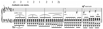
Example 1. Liszt, “Invocation,” mm. 1–5
(click to enlarge)
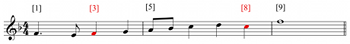
[1] In recent years, Franz Liszt has garnered increasing interest among music theorists for his innovations in harmony and form.(1) However, little attention has been given to rhythmic/metric aspects of his compositional style:(2) in particular, he frequently incorporates rich rhythmic structures in which the notated meter, given by time signatures and bar line placement, and the meter perceived by the listener are locked in an evolving conflict. Example 1, from Liszt’s “Invocation,” illustrates. A listener without access to the score would likely hear the first sounding chord as an opening downbeat, followed by several two-beat measures. A glance at the score, however, reveals that the opening “downbeat” is actually beat two; furthermore, the notated meter in the opening is not \(\substack{2\\4}\), but \(\substack{3\\4}\). While the sounding music does eventually fall in line with the notated \(\substack{3\\4}\) meter, the opening of the piece demonstrates a striking contrast between what the listener hears, or metrically entrains, and what is written.(3) These considerations suggest the presence of two distinct metrical layers: a layer supported by auditory cues in the sounding music and only indirectly implied by the musical notation, and an idealized layer represented by time signatures and barring that hearing alone may not reveal.
[2] At this point, one might be tempted, as a listener or performer, to prioritize one of these two layers. However, I argue that for performers and informed listeners, these layers form a larger, more complex musical experience than that provided by either layer on its own.(4) This perspective motivates an important question: how might relationships and interactions between conflicting metrical layers be modeled over the course of a piece when one layer is sonically articulated while the other is cognitively “internalized” by the informed listener? While the present article will focus on the music of Liszt, this question has broader relevance to innumerable Western and non-Western musical styles, from Brahms to Stravinsky to South Indian Carnatic music.(5)
[3] To differentiate between these two metric layers in discussion, I will tentatively call the internalized, referential metric layer the
[4] While these sorts of metric relationships have not been widely discussed in Liszt’s music, Krebs (1999) has thoroughly treated conflicts between metrical layers in Robert Schumann’s music. Whereas Krebs’s basic analytical units are the metrically consonant or dissonant states, however, Lewin’s (1987) concept of the generalized interval system (GIS) suggests searching for an alternative approach that emphasizes not points or states in a musical space, but the intervals and changes between these objects. This perspective forms the springboard for the current study, which will model the interactions between \(X\)- and \(Y\)-metric layers(7) in Liszt’s music using a newly defined GIS and will apply these ideas to two preliminary Liszt analyses.(8) As will become clear, Lewinian GIS theory permits a quantifiable approach to metric conflict that can account for arbitrarily long or short metric spans and can analyze larger conflicting structures in terms of subcomponents. Beyond drawing upon GIS theory for its intrinsic usefulness, the current project aims, in applying Lewin’s theories to rhythmic/metric study, to contribute to a generally underdeveloped side of GIS theory.(9)
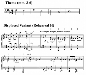
Example 2. Liszt, Totentanz, mm. 3–6 and rehearsal H. Dies irae theme and displaced variant
(click to enlarge)
[5] Example 2 presents another example of metric conflict, from Liszt’s Totentanz for piano and orchestra. At rehearsal H, Liszt begins a variant of the Dies irae theme on beat 2, and due to the phrasing and harmonic successions (e.g., the fermata and rest preceding the melody and the consistent appearance of local tonics on beat 2 and dominants on beat 1), beat 2 sounds like a downbeat and beat 1 an upbeat throughout the passage. In Krebs’s (1999) terminology, rather than a metrical “grouping dissonance” (31) like in Example 1, a “displacement dissonance” (33) of the form D2+1 (or D2−1) occurs. In other words, superimposed over the \(\substack{2\\4}\) \(X\)-meter is a conflicting \(Y\)-meter of \(\substack{2\\4}\)-shifted-by-one-beat. Although Krebs’s label is useful for describing the passage’s metrical state, it does not reveal how the music reached this displaced state, or what metrical processes might restore metrical consonance. In contrast, Lewin’s GIS machinery will allow not only differentiation between displaced and non-displaced metric states, but also representation of the dynamic shift in \(Y\)-downbeat location resulting from entering or leaving such a metrically displaced passage.
[6] It now deserves emphasis that the GIS to be developed in this article has a perceptual component, being partly based on auditorily derived metric interpretations. As such, applications of the GIS will draw upon Lerdahl and Jackendoff’s A Generative Theory of Tonal Music (1983). In this landmark work, the authors assert that meter is a concept broader than the simple barring on the page, defining metrical structure as “the regular, hierarchical pattern of beats to which the listener relates musical events” and describing how “phenomenal accents” in the score—cues such as dynamic changes, leaps, or harmonic changes—are key in creating a metric perception (17). Central to their metric theory is a set of four “metrical well-formedness rules” (MWFRs), which determine the set of “possible metrical structures” (68), and “metrical preference rules” (MPRs), through which a listener may choose among the possible metric interpretations for a musical passage (74). They note, however, that while MWFRs 1 and 2 are “common to all types of music,” MWFRs 3 and 4 may be “open to variation” or simply omitted (97).(10) Therefore, to accommodate metric hearings involving asymmetrical fives, sevens, and the like, the current project will omit MWFRs 3 and 4. Of the MPRs, the most important for the current study will be MPR 1 (Parallelism), which prefers that parallel musical groupings receive parallel metrical structures (75); MPR 2 (Strong Beat Early), which prefers that a musical group’s strongest beat appears early in the group (76); MPR 4 (Stress), which prefers metrical structures where accented notes are metrical strong beats (79); and MPR 5 (Length), which prefers metrical structures in which strong beats occur at the initiation of long pitch, dynamic, articulation, or harmonic events (84). Even when I do not reference these rules explicitly, they are at work in the background as I select metrical hearings for the Liszt works in question.
[7] Significantly, rather than taking Hasty’s (1997) moment-by-moment experiential approach, I will focus on what Lerdahl and Jackendoff (1983) call “the final state of [the listener’s] understanding” (4); namely, the metric structures being analyzed will be final metric interpretations for musical passages following careful reflection on the rhythmic and metric perceptions that the passages induce. “Final-state analysis” has not been free of criticism, however, as some have argued that this analytical mode reduces meter to a static, one-dimensional state and therefore inaccurately represents real-time metric processing.(11) Nevertheless, I adopt preference-rule-based final-state analysis for the current study because, as Temperley (2001) has argued, this approach can both model the unfolding listening experience quite well and allow for metrical revisions.
[8] Specifically, Temperley uses a “dynamic programming” model to connect preference-rule-based analysis to in-time listening: rather than requiring an entire piece to be heard before analytical decisions are made, this model “realizes a preference rule system in a ‘left-to-right’ fashion, so that at each point, the system has a preferred analysis of everything heard so far—analogous to the process of real-time listening to music” (2001, 19). Hence, the “final” metric interpretation is the result of a continual process that leaves room for reinterpretation while listening. Temperley’s approach to final-state analysis, which is less static than Lerdahl and Jackendoff’s original formulation, forms a natural connection to Lewin’s (2006) own nonlinear model of listening (see below).
2. Possible Objections
[9] Before proceeding, I briefly consider some potential criticisms of my analytic approach and assumptions about meter. London’s (2004) theory of meter, which is listener-centric to the highest degree, provides two major challenges to my approach. First, London assumes that “listeners do not normally have access to other, nonauditory information, such as a score or the scansion of song lyrics” (22). Second, while he concedes that “metrical dissonance” can occasionally be a useful metaphor, he argues that metrically conflicting passages can only be perceived in two ways: the listener may either “focus on either layer of activity, using it as the basis for their metric construal” or “derive a composite pattern from the two layers of rhythmic articulation” (104). In other words, one cannot perceive two simultaneous meters, but must either prioritize one metric layer or combine both layers into a single rhythmic/metric whole.
[10] In response to London’s claim that listeners do not usually have access to the score, thus undermining the significance of the notated meter, I argue that theorists, performers, and informed listeners in the Western tradition do depend on the score to help inform their metric experiences. In other words, while one can certainly derive metric interpretations from sounding events alone, this need not be the limit of metric experience. My perspective has precedent in the analytic work of Schachter (1999), who observes conflict in the Menuetto of Mozart’s String Quartet, K. 590, between the clear two-measure hypermeter of the opening fourteen-bar strain and a tonally motivated partitioning into two seven-bar phrases (95–96). While the former interpretation is easy to derive aurally, Schachter notes that the latter, conflicting interpretation is “accessible to anyone who can read a score and count measures. Yet how many listeners, including trained musicians, would become conscious of [the seven-measure spans] without consulting the score?” (97). Furthermore, Schachter suggests in a metrically conflicting Schumann passage that the meter that “governs this passage” is the previously established notated meter, and one should assume composers mean what they write “unless there is strong evidence to the contrary” (97–98). Samarotto (1999) takes a similar perspective in discussing his notion of “shadow meter,” in which “the main meter, the meter as written, casts a shadow, as it were, on a subsidiary, displaced meter which we are drawn to hear as real until it dissolves” (235; emphasis added).(12) Like Schachter, Samarotto pits a secondary perceived meter against a more dominant, previously established notated meter.
[11] Other studies challenge London’s claim through stronger assertions of the notated meter’s independent validity. For instance, in a cognitive study by Sloboda (1983), six pianists of diverse ability levels were asked to sight-read a series of melodies, two of which were merely different barrings of a single melody. The results showed that the performers consistently applied different expressive variations of accent and articulation to these two melodies, and none of the subjects even noticed that the second melody was a rebarred version of the first. Additionally, in the second experiment in Sloboda’s study, listeners were able to identify the meters the performers were attempting to convey with a high success rate. These results underscore how drastically the notated meter and barring can inform metric experience. Krebs (1999), too, treats the notated meter as an independent musical object. In his discussion of “subliminal” metrical dissonances, in which notated and heard metric layers conflict, he argues that it is up to the performer to ensure subliminal dissonances do not sound like metrical consonances (47). Significantly, in Krebs’s view, the notated metrical layer need not be previously auditorily established to be a valid metric object, as his analysis of the opening to the finale of Schumann’s Piano Sonata, op. 11, illustrates (50–51).
[12] The Totentanz example above provides additional support for the musical validity of the notated meter: in orchestral performances, the notated meter is generally indicated to the players and audience by a conductor. In particular, the metrically displaced passage in Example 2 aurally conflicts with the two-beat conducting pattern the audience and players see. By extension, in non-orchestral music, one might envision an “imaginary conductor” sustaining the underlying notated meter at all times, even when the sonically articulated meter departs from it.(13)
[13] As for London’s second claim that listeners cannot simultaneously experience two metric interpretations in Western music, Poudrier and Repp (2013) prominently challenge this perspective. Their study suggests that given simple enough polymetric configurations,(14) trained listeners can track beats in two different meters simultaneously. Moreover, this ability seems to improve with practice and special listening strategies, such as tapping the pulse in one layer while listening to the other layer (387–88). Lewin (2006) provides a more philosophical take on how the listener might perceive multiple meters, depicting the listening experience as dynamic and nonlinear. For Lewin, the listener constantly makes connections forward and backward in musical time, forming perceptions that change and even compete with one another during listening. Hence, with respect to a metrically conflicting passage, it follows that the listener might have a fluid experience in which neither metric layer is uniformly prioritized; instead, the layers’ local priority freely alternates, and the nature of this alteration could vary substantially between hearings and performances. In sum, if our musical minds are as active as Lewin suggests, then even a brief metric conflict (as might occur in Western music) has rich potential for complex, multi-layered hearings that take into account more than one metric interpretation.
[14] A final potential criticism of my approach involves the basic notions of meter and metric layer. In their diverse theories of meter, Krebs (1999), Lerdahl and Jackendoff (1983), Hasty (1997), London (2004), and Mirka (2009)(15) all assume that meter cannot be defined until at least three musical events or pulses, demarcating two distinct time spans, have occurred. For my theory, however, which mathematically defines
3. A Theory of Metric GISs
Example 3. S space with a quarter-note pulse
(click to enlarge)
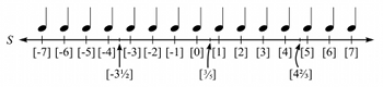
[15] Before attempting to model metric conflict using Lewin’s theories, I consider the simpler problem of defining a GIS that can measure intervals within a single metric layer. First, let \(S\) be the space described by Lewin (1987) as “a succession of time points pulsing at regular temporal distances one time unit apart” (22), and label each time point with an integer.(16) Furthermore, since traditional Western rhythmic notation is based on rational values (e.g., thirty-second notes or nested tuplets, but not
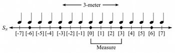
Example 4. Quarter-note S space endowed with 3-meter, where black dots represent downbeats
(click to enlarge)
[16] Furthermore, because the current study will investigate meter, I equip \(S\) with a constant \(n\)-meter corresponding to downbeats every \(n\) pulses for some integer \(n\).(17) A measure may then be defined as a span of \(S\) between consecutive downbeats, as shown in Example 4. The \(n\)-meter may also be interpreted locally rather than globally, so that meter changes (i.e., new distances between downbeats) are possible within \(S\).
Example 5. Quarter-note SN space where N = (2, 3[6], 5[12])
(click to enlarge)
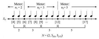
[17] I represent the total collection of meters in a piece by a metric succession N, given by
\[ N=\Big(n_1,{n_2}_{[r_2]},\dots,{n_k}_{[r_k]}\Big) \]
where meter \(n_2\) begins at some time point \([r_2]\), \([n_3]\) begins at \([r_3]\), and so forth. To allow this metric succession to encompass infinite \(S\) space, I assume that \(n_1\) extends from \([r_2]\) infinitely to the left, while \(n_k\) extends from \([r_k]\) infinitely to the right.(18) If a metric succession \(N\) is imposed on an \(S\) space, the resulting meter space may be called \(S_N\). \(S_N\) contains all time points of \(S\), but designates certain time points (determined by \(N\)) as downbeats. For instance, Example 5 depicts the space \(S_N\) where \(N=(2,3_{[6]},5_{[12]})\), implying 2-meter from \([6]\) infinitely to the left, 3-meter from \([6]\) to \([12]\), and 5-meter from \([12]\) onward. In situations where the \([r_i]\)’s are understood or not necessary for analysis, these subscripts may be omitted; thus, the metric list in the current example would simply be
Example 6. Brief melody in SN space, where N = (4)[1]
(click to enlarge)
Example 7. Brief melody in SN space, where N = (3)[1]
(click to enlarge)
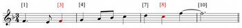
[18] Having defined the tentative GIS space \(S_N\), I now consider how to calculate intervals between time points. To motivate an appropriate interval function, I first consider the brief melody given in Example 6, which is in constant 4-meter with a quarter-note pulse and [1] as a downbeat. To define the rhythmic interval between [3] and [8], an obvious possibility would be \(int([3], [8]) = 8 - 3 = 5.\) However, Example 7 illustrates that placing the same melody in a new meter (3-meter) still yields \(int([3], [8]) = 8 - 3 = 5.\) Clearly, this tentative interval function is not sensitive to the meter values. Subtracting and then dividing by the respective meter values, however, accounts both for time points and for meter: \(int([3], [8]) = (8 - 3)/4 = 1\frac{1}{4}\) for the first example (4-meter), and \(int([3], [8]) = (8 - 3)/3 = 1\frac{2}{3}\) for the second example (3-meter). Intuitively, this division operation yields the same numerical result as counting measures in a given meter, as an orchestral player might: “ONE–two–three–four–TWO–two–three–four–THREE...” (how many full or partial measures result?). The new formula, then, is sensitive to metric context.(19)
Example 8. Passage with changing meter, where N = (3, 2[13])
(click to enlarge)
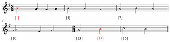
[19] However, consider the passage given in Example 8, where 3-meter (in half notes) gives way to 2-meter in m. 5. Suppose one wishes to calculate \(int([1],[14])\). While the meter change prevents application of the interval calculation in its current state, one can easily generalize \(int\) by calculating the number of measures lying between [1] and [14]. Numerically, this only requires “splitting” the interval calculation at the meter change, calculating the interval from [1] to [13]
Definition 1. Given a pulse space \(S\) endowed with a nonempty succession of meters \(N=\Big(n_1,{n_2}_{[r_2]},\dots,{n_k}_{[r_k]}\Big)\) where meters \(n_1\) and \(n_k\) extend infinitely to the left and right, respectively, then \[ GIS_N=(S_N,\,\mathbb{Q},\,int_N) \] where \(\mathbb{Q}\) is the additive group of rational numbers and \(int_N: S_N\times S_N\to \mathbb{Q}\) is defined as follows: if \(s\leq t\), \([s]\) is in meter \(n_j\), \([t]\) is in meter \(n_{j+x}\) for some \(x\geq 0\), and \(\{[r_{j+1}],\dots, [r_{j+x}]\}\) is the (possibly empty) set of meter changes between \([s]\) and \([t]\), then \[ int_N([s],[t])= \] \[ \frac{r_{j+1}-s}{n_j}+\frac{r_{j+2}-r_{j+1}}{n_{j+1}} + \cdots+\frac{r_{j+x}-r_{{j+(x-1)}}}{n_{j+(x-1)}} + \frac{t-r_{j+x}}{n_{j+x}}. \] If \(s>t\), then \[ int_N([s],[t])=-int_N([t],[s]). \]
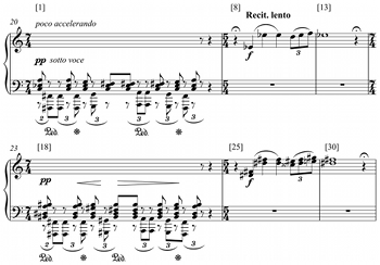
Example 9. Liszt, “Pensée des morts,” mm. 20–25
(click to enlarge)
[20] Essentially, this definition states that one can measure intervals in \(S_N\) by subtracting and dividing (as described above) within each metric region and then adding the results, and these intervals may be measured in a positive or negative direction. To clarify, consider the passage from Liszt’s “Pensée des morts” given in Example 9. Integer time points in this \(S_N\) space correspond to the quarter-note pulse, and the local metric succession is \(N = (7_{[1]}, 5_{[8]}, 7_{[18]}, 5_{[25]})\).(20) By Definition 1, then, the interval from [1] to [30] is \[ int_N([1], [30]) = \frac{8-1}{7} + \frac{18-8}{5} + \frac{25-18}{7} + \frac{30-25}{5} = 1+2+1+1 = 5. \] Thus, 5 measures occur between time points [1] and [30], as is easily verified in the score. Note, however, that shifting the intervallic endpoints by one pulse yields \(int_N([2],[31])=\frac{6}{7}+2+1+1\frac{1}{5}=\frac{6}{7}+4+\frac{1}{5}=5\frac{2}{35}\). This demonstrates that \(GIS_N\) intervals are highly contextual, for a simple shift by a pulse can result in a new interval. The notion of intervallic decomposition, to be defined in Section 4, will facilitate making contextual sense of seemingly unusual interval values like \(5\frac{2}{35}\) by breaking them into more intuitive numerical components.
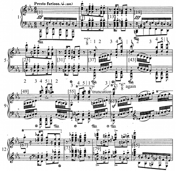
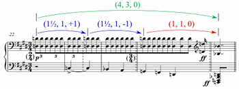
Example 10. Liszt, “Wilde Jagd,” mm. 1–15
(click to enlarge)
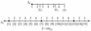
[21] Thus far, all calculations have implicitly depended on the metric layer corresponding to notated time signatures and bars—the \(X\)-layer. I have not, however, indicated how a conflicting \(Y\)-layer fits in. To approach this question, consider the span from [38] to [61] in Liszt’s “Wilde Jagd,” shown in Example 10. In this case, let \(S_X\) (i.e., \(S_N\) where \(N\) has been replaced by \(X\)) be eighth-note \(S\) space with constant meter \(X = (6)_{[1]}\). It then follows that \(int_X([38], [61]) = (61-38)/6 = 23/6 = 3\frac{5}{6}\).
[22] Also noteworthy, though, is the \(Y\)-meter as defined by sonically articulated cues and groupings. In the given passage, because the C minor chord at [38] sounds like a delayed (\(Y\)-)downbeat due to the eighth-rest on beat 1, and the initial rhythmic/melodic pattern repeats every five pulses, the start of each five-pulse group feels like the downbeat of a length-five measure. The consistent harmonic rhythm that alternates three-beat harmonies (longer) with two-beat harmonies (shorter) corroborates these downbeat locations.(21) Thus, time points [38] to [58] give the impression of 5-meter,(22) after which [61] abruptly returns to clear 6-meter, leaving the remaining span from [58] to [61], in final reflection, as an implied length-3 measure. In other words, the local \(Y\)-metric succession over this passage would be \(Y=(5_{[38]}, 3_{[58]}, 6_{[61]}).\) Definition 1, then, gives \(int_Y([38], [61]) = (58-38)/5 + (61-58)/3 = 4 + 1 = 5.\) From a more experiential perspective, the listener might start counting at [38], “ONE–two–three–four–five–TWO–two–three–four–five...”, ultimately finding that this counting is “cut off” by the apparent downbeat at [61]. Four \(Y\)-measures of length 5 and a lone length-3 \(Y\)-measure result, for a total of five \(Y\)-measures.
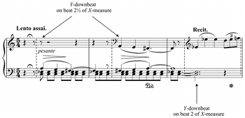
Example 11. Liszt, “Pensée des Morts,” mm. 1–3. Y-downbeat shift of -1/2 (dotted bar lines indicate Y-measures)
(click to enlarge)
Example 12. ℚ/5ℤ, with sample integer and fractional values
(click to enlarge)
Example 13. 6-meter SX and corresponding SB space, which represents an idealized length-6 measure (“1” = beat 1, “2” = beat 2, etc.)
(click to enlarge)
[23] While these differing \(int_X\) and \(int_Y\) values clearly help quantify the conflict between \(X\)- and \(Y\)-layers in some sense, the two intervals reside in separate conceptual worlds. It might be useful, then, to combine these two values into a single interval to depict the relationship between the metric layers. One simple solution would be to place the two values into an ordered pair, yielding \(int([38], [61]) = (3\frac{5}{6}, 5).\) However, the relationship between these independent values is still somewhat obscured. To understand the net result of the conflict between the \(X\)- and \(Y\)-layers, observe that while the \(Y\)-downbeat at [38] occurs on beat 2 of the \(X\)-measure, the \(Y\)-downbeat at [61] occurs on beat 1 of the \(X\)-measure. Thus, the \(Y\)-downbeat shifts by \(-1\) from [38] to [61], which suggests adding a third coordinate to the tentative interval: \(int([38], [61]) = (3\frac{5}{6}, 5, -1).\)
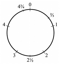
[24] Because the interval is now an ordered triple, it would make sense to combine \(GIS_X\) and \(GIS_Y\) (i.e., \(GIS_N\) for metric successions \(N=X\) and \(N=Y\)) with some sort of “downbeat shift GIS” to form a three-component direct product GIS.(23) Such a “downbeat shift GIS” would require a new downbeat shift space, interval group, and corresponding interval function. The interval group should be modular in some sense, and as depicted in Example 11, from Liszt’s “Pensée des morts,” it should be able to represent fractional \(Y\)-downbeat shifts as well as integer shifts. The additive group \(\mathbb{Q}/5\mathbb{Z}\), shown in Example 12, provides a potential solution in the case of “Pensée,” as this quotient group represents, informally, the additive “rationals mod 5.” Thus, for instance, in addition to being able to write \(3+4 = 7 \equiv 2\pmod{5}\), one may write \(2\frac{1}{3} + 10\frac{1}{3} = 12\frac{2}{3}\equiv 2\frac{2}{3}\pmod{5}\).
[25] Now, suppose a piece of music has constant \(X\)-meter \(m\), and I wish to define a tentative downbeat-shift GIS, \(GIS_B\). I may then define the GIS space as \[ S_B=[1, m+1)\cap\mathbb{Q} = \textrm{rational values }\geq 1\textrm{ and less than }m+1, \] which numerically represents beat locations in an idealized \(X\)-measure, as Example 13 illustrates. In this case, \(S_B\) is equal to \([1,7)\cap\mathbb{Q}\), the set of all rational beat locations \(b\) such that \(1\leq b<7\). Note that reaching 7 would be equivalent to reaching the next \(X\)-downbeat, or returning to beat 1.
[26] I therefore define the interval function for \(GIS_B\) to be \[ int_B(s,t)=t-s\pmod{m}, \] where \(s\) and \(t\) are rational locations within an \(m\)-beat measure. This function, applied to \(Y\)-downbeats, can calculate how far and in what direction the \(Y\)-downbeat shifts with respect to an \(m\)-beat \(X\)-measure. The resulting GIS, \(GIS_B=(S_B, int_B, \mathbb{Q}/m\mathbb{Z})\), suffices for analysis of music with constant \(X\)-meter, including much nineteenth-century music. This new GIS may be formally defined as follows:
Definition 2. Suppose \(S\) is a pulse space endowed with nonempty metric successions \(X=(m)\) and \(Y=(y_1,y_2,\dots,y_k).\) Then if \(S_B\) is the set of all possible rational beat locations within an idealized \(m\)-length measure, represented formally by \[ S_B=[1,m+1)\cap\mathbb{Q}, \] then \[ GIS_B=(S_B,\mathbb{Q}/m\mathbb{Z},int_B) \] where \(int_B\) is defined by \[ int_B(s,t)=t-s\pmod{m}. \]
Essentially, intervals between two \(Y\)-downbeat locations may be calculated via subtraction modulo the \(X\)-meter. To emphasize the dynamic nature of the \(Y\)-downbeat shift, I will label \(GIS_B\) intervals with a
[27] The chief limitation of \(GIS_B\) as given in Definition 2 is, of course, that it requires constant \(X\)-meter. Extending \(GIS_B\) to accommodate multiple \(X\)-meters, however, is challenging, as Lewin’s (1987) GIS definition requires a single interval group (26). Hence, one cannot simultaneously measure intervals in \(\mathbb{Q}/m_1\mathbb{Z}\) and \(\mathbb{Q}/m_2\mathbb{Z}\) where \(m_1\neq m_2\). For pieces with extended sections in different \(X\)-meters, one might sidestep the problem by simply applying \(GIS_B\) with the appropriate modulus value to each section. To measure intervals between these sections or apply \(GIS_B\) to pieces with frequent \(X\)-meter changes, though, an alternate formulation of \(GIS_B\) is necessary.
[28] Because the \(X\)-meter values in a piece could be as large as a composer desires, no finite modulus will suffice. Moreover, in pieces with rapidly changing \(X\)-meters (as in much twentieth- and twenty-first-century music), a single modular choice would miss the musical point. Thus, a logical solution is to reject modularity altogether and let \(S_B\) be an infinite “super-measure” containing all lengths of \(X\)-measure. One can still calculate intervals by subtracting beat locations, but the intervals will not be modularized; they will simply be elements of the additive group of rationals \(\mathbb{Q}\). Unlike in the modular case, however, \(S_B\) cannot have a leftmost boundary of 1. If it did, then a negative interval value could force an exit from the space, as one cannot reinterpret negative intervals as positive ones as in a modular interval group.
[29] This yields the following modified version of \(GIS_B\):
Definition 3. If \(S_B\) is an idealized infinite measure, represented formally by the set of rationals \(\mathbb{Q}\), then \[ GIS_B=(S_B,\mathbb{Q},int_B) \] where \(int_B\) is defined by \[ int_B(s,t)=t-s. \]
Note that the \(\mathbb{Q}\) in the second coordinate is the additive group of rationals, while \(S_B\) is simply a set. It is also important to recognize that \(GIS_B\) as defined here could have numerous analytic interpretations. For the current study, suppose one wishes to measure the interval between two \(Y\)-downbeats \([a]\) and \([b]\). Then one could imagine two copies of \(\mathbb{Q}\), one of which aligns with the \(X\)-measure containing \([a]\) such that the \(X\)-downbeat is labeled “1,” and the other of which similarly aligns with the \(X\)-measure containing \([b]\). Rational values for \([a]\) and \([b]\) may then be assigned according to the respective copies of \(\mathbb{Q}\); \(int_B\) will simply be the difference between these values. Effectively, then, \(Y\)-downbeat locations are subtracted as before, but without modularization.
[30] Having defined \(GIS_B\), I now construct the final, three-component direct-product GIS for analyzing metric conflict, which I call \(Met\). Two applications of definition 3.3.3 of GMIT (Lewin 1987, 45) are all that is needed.
Definition 4. Given a pulse space \(S\) endowed with nonempty metric successions \(X=(m_1,m_2,\dots,m_j)\) and \(Y=(y_1,y_2,\dots,y_k)\), then \[ Met=GIS_X\times GIS_Y\times GIS_B, \] with \(int_{Met}\) defined by \[ int_{Met}\Big(([x_1],[y_1],b_1), ([x_2],[y_2],b_2)\Big)= \] \[ \Big(int_X([x_1],[x_2]),int_Y([y_1],[y_2]),int_B(b_1,b_2)\Big). \]
In other words, points in \(Met\) are ordered triples consisting of a point from \(GIS_X\), a point from \(GIS_Y\), and a point from \(GIS_B\), and intervals are calculated one coordinate at a time (\(int_X\), \(int_Y\), \(int_B\)) to yield a new ordered triple. Also note that \(Met\) is contextually defined: namely, every pair of metric successions \(X\) and \(Y\) imposed on a space \(S\) generates a distinct GIS \(Met\).
Example 14. Met-based analysis summary
(click to enlarge)
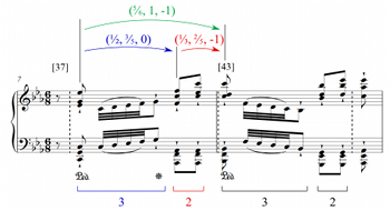
[31] As defined, \(Met\) is a large GIS, as all three coordinates represent independent parameters. Intuitively, given a set metric scheme, an arbitrary \(Met\) interval \[ (x,y,b)=\Big(int_X([x_1],[x_2]),int_Y([y_1],[y_2]),int_B(b_1,b_2)\Big) \] means that \(x\) \(X\)-measures occur from \([x_1]\) to \([x_2]\); \(y\) \(Y\)-measures occur from \([y_1]\) to \([y_2]\); and \(b\) beats (or a mod-\(m\) equivalent) transpire from beat location \(b_1\) to \(b_2\). Thus, the GIS is capable of handling three different independent measurements simultaneously, affording broad and diverse analytical possibilities. For the current study, rather than investigating each of these possibilities, I will focus on the application of \(Met\) suggested by Example 14, from the aforementioned conflicting region of “Wilde Jagd.”
[32] First, consider the interval between the opening C minor chord and the
[33] Additionally, observe how the two \((\frac{5}{6}, 1, -1)\) intervals(25) can be summed to form a larger \((1\frac{2}{3}, 2, -2)\) interval. Conversely, the latter interval can be decomposed into the former subintervals, an important GIS property that I explore in Section 4. As a final note, observe that the interval from \([48]\) to \([51]\), \((\frac{1}{2},\frac{3}{5},0)\), has a \(Y\)-downbeat shift of 0 (not \(+3\)) because both bounding time points are in the same \(Y\)-measure.
4. Intervallic Decompositions
Example 15. Liszt, “Invocation,” mm. 1–5 and 194–203. Y-decomposed Met intervals
(click to enlarge and see the rest)
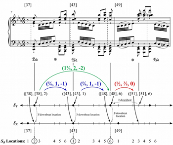
[34] Given that \(Met\) intervals can be measured between any two temporal locations in a piece, the number of distinct intervals available is staggering. To help make sense of this abundance of information, one might draw inspiration from the intervallic decomposition shown in Example 14: if an interval is broken into subintervals at \(Y\)-downbeats, then I call the resulting “prime factorization,” of sorts, the \(Y\)-decomposition of the original interval. Thus, the \(Y\)-decomposition of the uppermost, green interval in Example 14 is \[ \left(1\frac{2}{3},2,-2\right)=\left(\frac{5}{6},1,-1\right) +\left(\frac{5}{6},1,-1\right), \] or simply \[ \left(1\frac{2}{3},2,-2\right)=2\left(\frac{5}{6},1,-1\right). \] The \(Y\)-decomposition is significant in that it allows any interval to be broken into its basic components in a well-defined manner, facilitating meaningful comparisons between musical spans of arbitrary length. Example 15 illustrates an analytical application of this concept in Liszt’s “Invocation.” The first portion of the example shows the opening measures of the piece, which strongly suggest a \(\substack{2\\4}\) \(Y\)-meter in conflict with the \(\substack{3\\4}\) \(X\)-meter, as previously noted. Above the score, I translate this observation into \(Met\) intervals: the long, green arrow at the top shows that the interval across the entire conflicting span is \((2\frac {2}{3},4,-1)\), while the shorter, blue arrows break this larger interval into four \((\frac{2}{3}, 1, -1)\) subintervals, each spanning a single \(Y\)-measure.
[35] The second portion of Example 15 shows the end of the piece, where a left hand triplet pattern abruptly yields to an eighth-note pattern. While this change of beat division might seem abrupt, observe that the eighth-note pattern spans \(2\frac{2}{3}\) \(X\)-measures—precisely the same length as the metrically conflicting span in mm. 1–3. Thus, shifting from descriptive to suggestive analysis,(26) a \((2\frac{2}{3}, 4, -1)=4(\frac{2}{3}, 1, -1)\) interval might be imposed on this later passage, as indicated by the arrows. This yields a metrical hearing that not only makes sense of the seemingly awkward intrusion of the eighths, but also provides a connection to the piece’s opening measures. Consequently, the interval \((2\frac{2}{3},4,-1)=4(\frac{2}{3},1,-1)\), which I label \(I\) in subsequent discussions, becomes a sort of intervallic bookend for the piece.(27)
Example 16. Liszt,
(click to enlarge)
[36] The \(Y\)-decomposition has a major weakness, however: it is not sensitive to metrical “displacement dissonances” (Krebs 1999, 33). Example 16 returns to the Totentanz passage from Example 2, this time with \(Met\)-intervallic annotations. Observe that the passage preceding rehearsal H is in non-displaced \(\substack{2\\4}\) meter, while the passage following H is metrically displaced one beat to the right. Between the fermata and the entry after H, the \(Y\)-downbeat shifts by \(+1\).(28) The metrically displaced state after H could thus be viewed as the result of a dynamic shift of the \(Y\)-downbeat. Nevertheless, the \(Y\)-decomposed \(Met\) intervals within each metric region are identical: two measures of aligned \(\substack{2\\4}\) and two measures of displaced \(\substack{2\\4}\) both span the interval \((2,2,0)=2(1,1,0)\).
Example 17. Liszt, Totentanz, rehearsal H. X-decomposition illustrated
(click to enlarge)
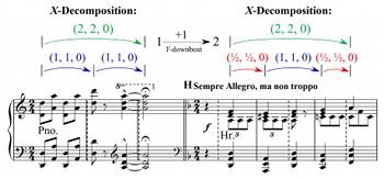
[37] To address this weakness, I introduce a new intervallic decomposition, the \(X\)-decomposition, that breaks down intervals at \(X\)-downbeats. Example 17 illustrates. Note that while two measures of aligned \(\substack{2\\4}\) meter have \(X\)-decomposition \((2,2,0)=2(1,1,0)\), two measures of displaced \(\substack{2\\4}\) decompose as \((2,2,0)=(\frac{1}{2},\frac{1}{2},0)+(1,1,0)+(\frac{1}{2},\frac{1}{2},0)\). Thus, the \(X\)-decomposition highlights the contextual metrical differences between the two passages.
Example 18. Liszt, Totentanz, rehearsal H. XY-decomposition illustrated
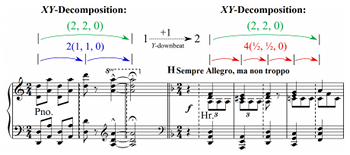
(click to enlarge)
[38] A third and final type of decomposition combines the advantages of both \(X\)- and \(Y\)-decompositions: the \(XY\)-decomposition breaks down intervals at \(X\)- and \(Y\)-downbeats, as shown in Example 18. In this case, while the passage before H still decomposes as \((2,2,0)=2(1,1,0)\), the displaced passage now breaks down as \((2,2,0)=4(\frac{1}{2},\frac{1}{2},0)\). Observe that a new subinterval begins each time a dotted or solid bar line appears. Significantly, this decomposition not only differentiates between aligned and displaced metric states, but can actually be nested within the \(X\)- and \(Y\)-decompositions. For instance, combining the middle two subintervals after H yields the \(X\)-decomposition, while combining the first two and final two subintervals produces the \(Y\)-decomposition.
[39] While the \(X\)-, \(Y\)-, and \(XY\)-decompositions are the only intervallic decompositions I formally define here, many other types of decomposition are possible. For instance, the “Wilde Jagd” analysis in Section 6 breaks down selected intervals according to harmonic rhythm, yielding intervallic decompositions that do not correspond to \(X\)-, \(Y\)-, or \(XY\)-decompositions. Intervals might also be decomposed according to articulation, phrasing, rhythmic characteristics, and other non-metric parameters. In general, the type of decomposition chosen will depend on analytical context.
5. Intervallic Expansions and Contractions
Example 19. Several transformations of a Met interval, generated by traditional augmentation and diminution
(click to enlarge)
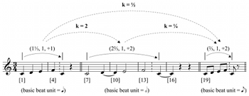
[40] While \(Met\) intervals are analytically useful as defined, it would be well within the spirit of a Lewinian project to determine how characteristic \(Met\) intervals can appear at multiple hierarchical levels.(29) In other words, it could be valuable to investigate what happens to a given interval when a passage’s analytical pulse unit is altered. Traditional augmentation and diminution provide a familiar example, as shown in Example 19, which depicts the pulse unit of a simple melody expanding and contracting by the indicated \(k\)-values. Note that each interval spans one \(Y\)-measure, but the melody’s analytical beat unit changes from quarter note to half note to eighth note over the course of the example.
Example 20. Liszt, “Wilde Jagd,” mm. 7–9 and 16–21. Intervallic expansion
(click to enlarge)
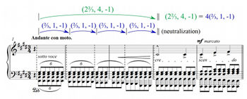
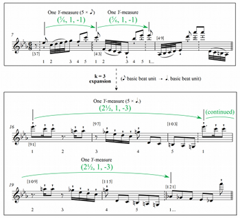
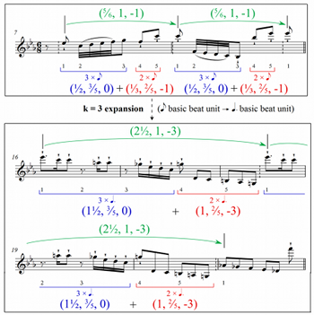
[41] Observe, though, that the specific melodic pitches and rhythms do not affect the \(Met\) intervals in any way. This suggests generalizing beyond traditional augmentation and diminution by, say, expanding three \(Y\)-measures at the quarter-note level to three \(Y\)-measures at the half-note level, or contracting four \(Y\)-measures at the half-note level to four \(Y\)-measures at the eighth-note level, but not necessarily preserving melody or rhythm. The passages in Example 20 from “Wilde Jagd” illustrate this idea. Intuitively, this diagram shows two five-eighth-note \(Y\)-measures in mm. 7–8 expanding to two five-dotted-quarter-note \(Y\)-measures in mm. 16–21. In the process, two consecutive \((\frac{5}{6}, 1, -1)\) intervals expand by a factor of \(k=3\) to produce two \((2\frac{1}{2}, 1, -3)\) intervals. At this point, though, one might be skeptical about how musically significant or revealing this relationship is.
[42] Before investigating this point, I consider intervallic contraction and expansion from a more formal perspective. First, it is worth noting that the relationships I am describing do not correspond to Krebs’s (1999) metrical dissonance “families” in which the grouping dissonance Gx/y is in the same family as G2x/2y, G3x/3y, etc., and the displacement dissonance Dx+a is in the same family as D2x+2a, D3x+3a, and so forth (41–42). In particular, each of these families represents a single ratio between conflicting layers. Observe, however, that this is not what occurs in Example 19. In Krebs’s notation, where “1” represents the quarter note, the first interval spans a G4/3 grouping dissonance; the second spans G8/3; and the final interval represents G3/2. Note that each of these is in a different Krebsian family of grouping dissonances. The essential difference between Krebs’s expansions/contractions and mine is that Krebs expands/contracts both layers by the same factor, while I only expand/contract a single layer (the \(Y\)-layer) while keeping the other layer (the \(X\)-layer) unchanged, resulting in new forms of conflict.
[43] While the most general mathematical formulation of these ideas is rather involved,(30) the following proposition provides a numerical method for expanding and contracting \(Met\) intervals that covers most of the cases relevant to the current study. In this proposition, the notation \(I_{[s][t]}\) is shorthand for “the \(Met\) interval from \([s]\in S\) to \([t]\in S\).” For instance, \(I_{[1][4]}\) means \[ int_{Met}\Big(([1],[1],B[1]),([4],[4],B[4])\Big), \] where \(B[s]\in S_B\) is the \(Y\)-downbeat location of the \(Y\)-measure containing \([s]\).
Proposition 1. Let \(S\) be a pulse space endowed with nonempty metric successions \(X=(m)\) and \(Y\). For some rational \(x,y\geq 0\), suppose the \(Met\) interval \((x,y,a)\) can be expressed as \(I_{[s][t]}\) for \(Y\)-downbeats \([s]\) and \([t]\). Then for any positive rational \(k\), the \(k\)-expansion/contraction of \((x,y,a)\) is given by \[ (kx, y, kxm). \]
[44] Observe that to apply this proposition, the transformed interval must begin and end at \(Y\)-downbeats, and \(k\) may be any positive rational. If \(k\) is an integer, though, the calculation becomes simpler and does not require the transformed interval to begin and end at \(Y\)-downbeats:
Proposition 2. Let \(S\) be a pulse space endowed with nonempty metric successions \(X=(m)\) and \(Y\). For some rational \(x,y\geq 0\), suppose the \(Met\) interval \((x,y,a)\) can be expressed as \(I_{[s][t]}\) for \([s],[t]\in S\), not necessarily \(Y\)-downbeats. Then for any positive integer \(k\), the \(k\)-expansion of \((x,y,a)\) is given by \[ (kx, y, ka). \]
For instance, Proposition 2 implies that the 3-expansion of the \((\frac{5}{6},1,-1)\) interval from Example 20 is \[ \left(3\left(\frac{5}{6}\right), 1, 3(-1)\right)=\left(2\frac{1}{2}, 1, -3\right). \] Equivalently, since \((\frac{5}{6}, 1, -1)=(\frac{5}{6}, 1, +5)\) in constant 6-meter (\(X=(6)\)), calculation shows that \((\frac{5}{6}, 1, +5)\) expands to \[ \left(3\left(\frac{5}{6}\right), 1, 3(+5)\right)=\left(2\frac{1}{2}, 1, +3\right). \]
[45] At this point, it is worth pausing to reflect critically on the system being developed. Given the density of technical mathematical details, one might question whether these intricate \(Met\) intervals are really necessary. For instance, in Example 20, one might reasonably argue that the 3-expansion here could simply be described as two heard five-eighth-note measures expanding to two heard five-dotted-quarter-note measures. True as this may be, the \(Met\) intervals in the example, \((\frac{5}{6},1,-1)\) and \((2\frac{1}{2},1,-3)\), represent more. In particular, suppose that Liszt had notated the upper passage in \(\substack{5\\8}\) and the lower passage in \(\substack{15\\8}\). This, too, would involve two heard five-eighth-note measures expanding to two heard five-dotted-quarter-note measures, but all of the resulting \(Met\) intervals would be \((1,1,0)\). The fact that the intervals are not all \((1, 1, 0)\) and, in fact, change substantially in the expansion suggests that an altered pulse unit is only part of the picture. Indeed, to fully understand these passages’ role in the context of the piece, one must consider how an idiosyncratic, evolving conflict with the underlying \(\substack{6\\8}\) meter affects the musical experience. This, precisely, is what the \(Met\) intervals are intended to represent.
[46] It is also worth noting that many relatively trivial relationships can be numerically represented by intervallic expansions and contractions. For instance, a measure without metric conflict, spanning \((1,1,0)\), technically 2-expands to a two-bar hypermeasure, spanning \((2,1,0)\). Because such relationships will inevitably be found in most nineteenth-century works, I close this section with a set of criteria for identifying nontrivial expansions and contractions for the current project:
- At least one of the intervals in the expansion/contraction relationship must span a metrically conflicting region (e.g., a subliminal grouping or displacement dissonance, in Krebs’s terminology).
- An expansion/contraction relationship is strengthened if the intervals in question are consecutive or close together in the piece.
- One or both intervals in the relationship should be distinctive or idiosyncratic. For instance, an interval might occur or recur in a piece in marked ways, span \(Y\)-measures of unusual lengths (e.g., five or seven beats), or have a characteristic decomposition that is preserved in the expansion/contraction.
These criteria are implicitly at work in the following section’s analyses, which will highlight distinctive intervallic expansions and contractions in Liszt’s “Wilde Jagd” and “Invocation.”
6. Two Abbreviated Liszt Analyses
Example 21. Liszt, “Wilde Jagd,” mm. 7–8. Intervallic decomposition of W = (⅚, 1, −1)
(click to enlarge)
Example 22. Liszt, “Wilde Jagd,” mm. 7–8 and 16–21. Y-decomposition-preserving 3-expansion
(click to enlarge)
Example 23. Liszt, “Wilde Jagd,” mm. 7–8 and 11–15. Intervallic 6-expansion of W
(click to enlarge)
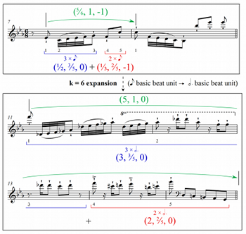
[47] With all of the requisite analytical machinery in place, I now examine more deeply the musical workings of mm. 1–21 of “Wilde Jagd.” I begin with the simple observation that the harmonic rhythm of the five-beat \(Y\)-measures starting at [38] suggests a consistent 3+2 partitioning, motivating the decomposition of \((\frac{5}{6},1,-1)\) shown in Example 21. For the remainder of this analysis, I call this interval, with its characteristic decomposition, \(W\) (for “wild”). I now expand \(W\), and its subintervals, to two higher hierarchical levels—namely, the dotted-quarter-note and dotted-half-note levels. Multiplying the first and third coordinates of each interval by the corresponding expansion factors of 3 and 6, respectively (Proposition 2), demonstrates that \[ W=\left(\frac{5}{6}, 1, -1\right)=\left(\frac{1}{2}, \frac{3}{5}, 0\right) +\left(\frac{1}{3}, \frac{2}{5}, -1\right) \] 3-expands to \[ W_3=\left(2\frac{1}{2}, 1, -3\right)=\left(1\frac{1}{2}, \frac{3}{5}, 0\right) +\left(1, \frac{2}{5}, -3\right) \tag{2} \] and 6-expands to \[ W_6=\left(5, 1, 0\right)=\left(3, \frac{3}{5}, 0\right) +\left(2, \frac{2}{5}, 0\right). \tag{3} \] An interesting question, then, is whether the theoretical decomposition in (2) can be applied to the musical 3-expansion from Example 20. Example 22 illustrates that this is, indeed, the case, for the passage beginning at m. 16 exhibits 3+2 melodic-harmonic groupings at the dotted-quarter-note level. This observation gives special musical significance to the previously observed 3-expansion of \(W\) at m. 16.
[48] Also noteworthy is that while the two \((\frac{5}{6},1,-1)\) intervals combine to yield \((1\frac{2}{3},2,-2)\), an interval with a \(-2\) \(Y\)-downbeat shift, the two \((2\frac{1}{2},1,-3)\) intervals combine into \((5, 2, -6)=(5, 2, 0)\). Thus, while \(2W (=W+W)\) accomplishes a nonzero net \(Y\)-downbeat shift, the 3-expansion \(2W_3\) does not, demonstrating a substantial change in local metric conflict due to the expansion. Significantly, at m. 16, Liszt uses the minimum number of \(W_3\) intervals (two) necessary to execute a net zero \(Y\)-downbeat shift.
[49] Now, while I have considered mm. 7–10 and 16–20, I have thus far disregarded mm. 11–15: might this passage contain some kind of expansion of \(W\) as well? As Example 23 illustrates, this is indeed the case, for if the entire span of mm. 11–15 is heard as a single hypermeasure (specifically, a five-beat \(Y\)-measure where the beat unit is a dotted half note), then this passage not only represents an expansion of \(W\), but again exhibits the characteristic 3+2 partitioning (three measures of
[50] A few comments are in order regarding analytical methodology here. First, it is conceivable that one could locate these expansions of \(W\) in an ad hoc fashion, searching for 3+2 patterns at various levels of structure without using \(Met\). However, the purpose of the \(Met\) intervals is to depict not just 3+2 recursion, but the expressive effect of this recursion against the constant \(X\)-meter. Second, in locating these “Wilde Jagd” intervals, my working method was numerically grounded: I would first calculate an abstract expansion of \(W\), and then would determine if the resulting interval might be musically manifested. The \(int_X\) values were particularly useful in this regard; for instance, after calculating the 3-expansion of \(W\), I searched for \(2\frac{1}{2}\)-measure spans of music that could serve as \(Y\)-metric units and partition into \(1\frac{1}{2}\) measures + 1 measure, leading to the finding in Example 22. As such, the numerical expansion techniques are not only descriptively powerful, but useful for teasing out metric relationships that may not be immediately obvious.
Example 24. Liszt, “Wilde Jagd,” mm. 1–20. Overall path of interval W = (⅚, 1, −1)
(click to enlarge and see the rest)
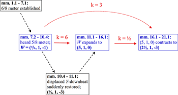
[51] Example 24 summarizes the progress of the characteristic interval \(W=(\frac{5}{6},1,-1)\) through the opening section of “Wilde Jagd.” As indicated in the example, Liszt establishes \(\substack{6\\8}\) meter over the first six measures and then, in mm. 7–10, introduces the \(\substack{5\\8}\) \(Y\)-meter that generates \(W\) for the first time. Then, after the \(Y\)-downbeat is suddenly brought back to beat 1 of the \(X\)-measure at the start of m. 11, generating the new interval \((\frac{1}{2},1,-3)\), the subsequent passage 6-expands \(W\), yielding \(W_6=(5,1,0)\). Following this five-measure passage, the expanded interval is in turn contracted by a factor of \(k=\frac{1}{2}\) to yield the 3-expansion of \(W\), \(W_3=(2\frac{1}{2},1,-3)\). Once again, note that the expansions and contractions across the central blue boxes preserve the characteristic decomposition of the original interval. Also significant is that the \(Y\)-downbeat shift values, which reflect interactions between \(X\)- and \(Y\)-layers, progress from a small shift
Example 25. Introduction of the interval J = (3, 4, 0) = 3(⅔, 1, −1) + (1, 1, 0)
(click to enlarge and see the rest)
Example 26. Liszt, “Invocation,” mm. 22–25 and 133–42. A 3-expansion of J = (3, 4, 0) = 3(⅔, 1, −1) + (1, 1, 0) at the recapitulation of the opening theme, spanning the surge to a dramatic climax in m. 142
(click to enlarge)
Example 27. Liszt, “Invocation,” mm. 52–57 and 155–67. The first statement of the chorale theme, the cadenza, and the second statement of the chorale theme in tonic. The cadenza spans another 3-expansion of J
(click to enlarge and see the rest)
Example 28. Summary of key intervallic events and transformations in Liszt’s “Invocation”
(click to enlarge)
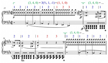
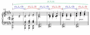
[52] While the preceding analysis has shown how metric conflict can shape a short section of a piece, I now demonstrate how \(Met\)-intervallic relationships can function on a larger scale through a brief analysis of Liszt’s “Invocation” from Harmonies poétiques et religieuses, S. 173. Recall that Example 15 indicated the importance of the interval \[ I=\left(2\frac{2}{3},4,-1\right)=4\left(\frac{2}{3}, 1, -1\right) \] as a sort of “bookend” for the piece. While this interval and the related interval \(K=(2,3,0)=3(\frac{2}{3}, 1, -1)\)—essentially, a truncation of \(I\) by one \(Y\)-measure—appear throughout the piece (mm. 12–14, 81–92, 117–18, 123–24, etc.) and thus serve as a unifying device, another interval will form the focus of the present discussion. This interval first appears in mm. 22–24, where right hand triplets that recall the opening are followed by an accented left hand note, which is tied over the bar line, as shown in Example 25. The result is a series of three \(Y\)-measures of length 2. Unlike in the opening, though, there is not a fourth length-2 \(Y\)-measure, as the next feeling of downbeat does not occur until the start of m. 25. Thus, a \(\substack{3\\4}\) \(Y\)-measure results that temporarily aligns with the \(X\)-meter. It follows that the interval spanning mm. 22–25.1, \(Y\)-decomposed, is \((3, 4, 0)=3(\frac{2}{3}, 1, -1)+(1,1,0)\). I call this interval, with its characteristic \(Y\)-decomposition, \(J\).(32)
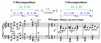
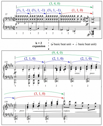
[53] Example 25 then shows how \(J\) is immediately manifested three more times over mm. 25–33, once for each phrase. While the interval makes several other literal appearances over the course of the piece when the thematic material from mm. 22–33 reappears in various forms, I now shift focus to some less obvious instantiations—namely, two intervallic expansions that occur at crucial points in the piece. Example 26 shows how in the recapitulation of the opening theme starting at m. 133, the measures leading to a climactic moment at m. 142 could be heard as three \(\substack{6\\4}\) \(Y\)-measures followed by one \(\substack{9\\4}\) \(Y\)-measure. This observation generates the interval \[ (9,4,0)=3(2,1,0)+(3,1,0), \] which is precisely the \(Y\)-decomposition-preserving 3-expansion of \(J\) (\(J_3\)). Observe as well that at this level of expansion, all \(Y\)-downbeat shift values are neutralized to 0. Significantly, this new interval \(J_3\) spans the entire push to the climax in m. 142 and allows the final three-measure unit to be viewed not merely as an isolated phrase extension, but as an outgrowth of earlier metric phenomena.
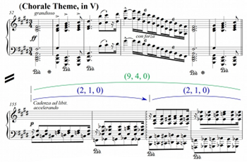
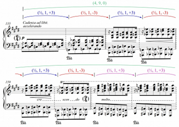
[54] A few measures later (m. 147), Liszt provides a brief return to the original, non-expanded \(J\) interval, followed by an extended variant of \(J\). Shortly thereafter, the cadenza in m. 155–63 strongly suggests another instance of \(J_3=(9,4,0)=3(2,1,0)+(3,1,0)\), as shown in Example 27. Significantly, the ultimate goal of this cadenza is the return of a majestic chorale theme that previously appeared in the dominant key and now appears in tonic, shortly before the end of the piece.(33) Thus, the expanded \(J\) here pushes toward a critical thematic and tonal moment.
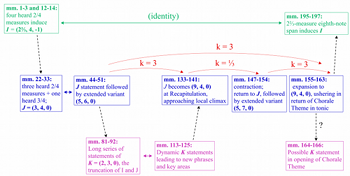
[55] Example 28 summarizes the transformations of the intervals \(I\), \(J\), and \(K\) across the piece, including some transformations I have not explicitly discussed in this abbreviated analysis. Significantly, the diagram shows how the metric conflict introduced in the opening pages of the piece serves as a shaping force for the remainder of the piece. Additionally, while the interval \(I\) seems to represent opening and closure, \(J\) is associated with development and mobility. The interval \(K=(2,3,0)=3(\frac{2}{3},1,-1)\), which I have not discussed in detail, can be thought of as the common portion of \(I\) and \(J\) (three two-beat \(Y\)-measures), thus serving as a unifying interval. In sum, this analysis illustrates how evolving metric conflict can impact not only local musical relationships, as in the “Wilde Jagd” analysis, but also global ones.(34)
7. Met Analysis Reconsidered: Interchanging X and Y
[56] The analyses thus far have consistently assumed that \(X\) represents the notated meter and \(Y\) the heard meter (or quasi-metrical effect). Indeed, letting written time signatures define the \(X\)-layer ordinarily makes sense, as traditional music reading occurs with reference to the notated measures. Technically, though, there is nothing preventing \(X\) from representing the heard meter and \(Y\) the meter given by the notated barring. This alternative perspective reifies the heard meter in a way that my previous interpretation of \(Met\) does not, as the heard metric layer becomes the referential layer against which the notated downbeat can “shift.”(35) This new perspective is not a mere theoretical abstraction, but is musically cogent, for the aural immediacy (by definition) of the heard metric layer makes it a useful reference for the less tangible notated metric layer. Moreover, this perspective can suggest new theoretical observations to complement the previous section’s metrical analyses. To demonstrate, I return briefly to “Invocation” and “Wilde Jagd.”
Example 29. Liszt, “Invocation,” mm. 22–25. A new set of intervals resulting from swapped interpretations of X and Y
(click to enlarge)
[57] First, with respect to “Invocation,” recall that the interval \(J=(3,4,0)=3(\frac{2}{3},1,-1)+(1,1,0)\) from the original analysis was particularly significant due to its expansions and contractions at key moments. Example 29 shows mm. 22–25, where \(J\) first appeared, but with the roles of \(X\) and \(Y\) interchanged as described above. The excerpt has been rebarred accordingly so that solid bar lines (\(X\)-measures) now correspond to heard measures while dotted bar lines (\(Y\)-measures) correspond to Liszt’s notated measures. In this example, the time signatures in parentheses correspond to the \(X\)-meter (heard meter; solid bar lines). What results is a new interval \[ J’=(4,3,0) = \left(1\frac{1}{2},1,+1\right) + \left(1\frac{1}{2},1,-1\right) + (1,1,0). \] Note that because the \(X\)-meter over this passage is non-constant, I calculate the \(Y\)-downbeat shift via non-modular subtraction: \(2-1=+1\) and \(1-2=-1\) (see discussion preceding Definition 3 in Section 3).
Example 30. Liszt, “Invocation,” mm. 133–42. Reversed meanings of X and Y drastically increase the number of components in the Y-decomposition
(click to enlarge and see the rest)
[58] Now, recall that the primary \(J\)-expansion in the original analysis was \[ J_3=(9,4,0) = 3(2, 1, 0) + (3, 1, 0), \] which first occurs at the recapitulation of the opening theme at m. 133. As Example 30 shows, however, the \(Met\) interval occurring when \(X\) and \(Y\) are reversed cannot be generated by simply expanding \(J’\) and its subintervals. In particular, while \(J’\) has three components in its \(Y\)-decomposition, this new interval has a nine-component decomposition, which can be written compactly as follows: \[ (4,9,0)=3\left[\left(\frac{1}{2},1,+3\right)+\left(\frac{1}{2},1,-3\right)\right] + 2\left(\frac{1}{3},1,+3\right)+\left(\frac{1}{3},1,-6\right). \tag{4} \]
[59] As such, the transformation of \(J’\) into \((4,9,0)\) is not an intervallic expansion as defined in Section 5, even though the \(X\)-meter values in mm. 22–25 (2, 2, 2, 3) can be augmented by a factor of 3 to yield the values over mm. 133–42 (6, 6, 6, 9). Again, the augmentation alone is not my primary concern, but rather the metric conflict that such a procedure generates. In this regard, as the \(X\)-meter is augmented, the \(Y\)-meter remains a constant 3, producing the large number of components appearing in the \(Y\)-decomposition.
[60] While the decomposed interval in (4) is much less elegant than \[ J_3=(9,4,0) = 3(2, 1, 0) + (3, 1, 0) \] from the original analysis, it also provides new analytical possibilities that \(J_3\) misses. For instance, a glaring weakness of \(J_3\) is the lack of activity in the \(int_B\) coordinates, as the expansion has reached a hierarchical level where \(X\)- and \(Y\)-downbeats align, neutralizing \(Y\)-downbeat shifts. The new decomposition in Example 30, however, is extremely sensitive to the relationship between \(X\)- and \(Y\)-downbeats, providing a useful picture of the metrical ebb and flow. Specifically, while each “\(+\)”-valued interval pulls the \(Y\)-downbeat away from the \(X\)-downbeat, each “\(-\)”-valued interval restores downbeat alignment. In a pseudo-energeticist vein, one might read the “\(+\)” intervals as building potential energy and the “\(-\)” intervals as releasing kinetic energy.(36)
[61] This reading is particularly compelling at m. 139. First, observe that each of the three preceding \(X\)-measures enacts an “energy”-building \(+3\) \(Y\)-downbeat shift followed by a \(-3\) shift that releases this energy, restoring the alignment of \(X\)- and \(Y\)-downbeats. The nine-beat \(X\)-measure at m. 139 initially appears to continue this pattern, starting with a potential-energy-increasing \(+3\) shift. However, what follows is not a release, but another energy-building \(+3\) shift. Thus, metrical realignment at m. 142 requires the \(Y\)-downbeat to release the accumulated energy by shifting by \(-6\). This delayed energy release, whose magnitude is double what occurred in the previous \(X\)-measures, helps push the music into the previously discussed climax at m. 142.
[62] Obviously, there are major limitations to this pseudo-energetic metaphor, for perhaps it is silly to claim that in a nine-beat measure, beat 6 is farther from the downbeat than beat 3. Similarly, can one reasonably claim that a net \(+6\) \(Y\)-downbeat shift builds more potential energy than a \(+3\) shift? While one perhaps cannot make this claim in general, the metaphor and its relation to the \(int_B\) values seem quite apt in this passage’s context, due to the passage’s melodic structure and overall direction. Furthermore, this interpretation suggests an element of metric flux within the heard measures that the original \(J\)-based analysis missed.
Example 31. Liszt, “Invocation,” mm. 155–66. (4, 9, 0) in rebarred cadenza
(click to enlarge and see the rest)
[63] One could make similar observations in the cadenza, where the original analysis located another \(J_3\) interval leading into the climactic return of the chorale theme in tonic. As shown in Example 31, another \((4,9,0)\) interval appears, again containing an internal ebb and flow of \(Y\)-downbeat shifts. In this case, the surge of energy embodied by the \(\substack{9\\4}\) \(X\)-measure carries the piece into its tonal resolution, where the chorale theme—previously presented in V—occurs in I. While I referenced this surge of energy in my earlier analysis, the final \(Y\)-downbeat-shift sequence of “\(+3\), \(+3\), \(-6\)” makes the image of intensifying and released energy even more vivid.
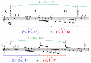
Example 32. Liszt, “Wilde Jagd,” mm. 16–21 (rebarred). The partitioning of two X-measures into 3+2 subdivisions
(click to enlarge)
[64] I now similarly revisit passages in “Wilde Jagd” containing expansions of the characteristic interval \(W=(\frac{5}{6}, 1, -1)\) from this new vantage point, thereby enriching and deepening the analytical results from Section 6. Consider, for instance, the passage where I originally located \(W_3\) (mm. 16–21; see Example 22). Example 32 illustrates the new \(X\)-decomposition above the staff, while the intervals induced by the characteristic 3+2 \(X\)-measure subdivisions appear below the staff. The example also labels \(Y\)-downbeat locations for clarity (note that \(S_B\) is locally fifteen-beat space). While the two consecutive occurrences of the interval \[ \left(2\frac{1}{2},1,-3\right)=\left(1\frac{1}{2},\frac{3}{5},0\right)+\left(1,\frac{2}{5},-3\right) \] in the original analysis emphasized parallelism between the passage’s two halves, this new analysis highlights non-parallel aspects based on metric context. The green intervals above the staff do maintain a sense of parallelism, as the \(int_X\) and \(int_Y\) values are equal and the \(int_B\) coordinates are additive inverses (\(\pm12\)). The symmetry of \(int_B\) values is lost, however, in the 3+2 decompositions, for while the first two subintervals have \(Y\)-downbeat shifts of \(+6\), the final two have values of \(-3\) and \(-9\), respectively. The \(-9\) is easily explained since \(-9\equiv +6\pmod{15}\), and 15 is the local \(X\)-meter. Thus, were the \(X\)-meter for the piece a constant 15, one could rewrite the final \((\frac{2}{5},1,-9)\) subinterval as another \((\frac{2}{5},1,+6)\). The \((\frac{3}{5},1\frac{1}{2},-3)\) subinterval is more curious, however, as \(-3\) is not equivalent to \(+6\) modulo 15. Apparently, the musical span that generates this subinterval differs in some essential way from the other bracketed spans.
[65] As depicted in Example 32, this difference stems from the \(Y\)-bar lines spanned: while the first, second, and fourth subintervals all cross over a single \(Y\)-bar line, the third subinterval crosses over two. Because \(Y\)-downbeats can only shift when the music crosses a \(Y\)-bar line, the two crossed bar lines enable two \(Y\)-downbeat shifts. In this case, the \((\frac{3}{5},1\frac{1}{2},-3)\) interval encompasses two nonzero \(Y\)-downbeat shifts, as the interval’s \(Y\)-decomposition clarifies: \[ \left(\frac{3}{5},1\frac{1}{2},-3\right) = \left(\frac{1}{5},\frac{1}{2},-9\right)+\left(\frac{2}{5},1,+6\right). \] In other words, the overall \(Y\)-downbeat shift of \(-3\) results from a \(-9\) shift followed by a \(+6\) shift, which would be equivalent to two \(+6\) shifts modulo 15. Thus, the current section’s new analytical perspective demonstrates how surface parallelism conceals underlying metric asymmetries, providing a richer understanding of this passage’s metric subtleties.
8. Final Thoughts
[66] To conclude, this study has provided but a glimpse of the compelling ways in which evolving metric conflict can function structurally and expressively in the music of Liszt, as well as showcasing the capabilities of \(Met\) for metric analysis. In the initial analysis of “Wilde Jagd,” I suggested how the recurring interval \(W=(\frac{5}{6}, 1, -1)\) plays an important role in the first section of the etude and, as further analysis can show, in the remainder of the piece. Moreover, because of the metric asymmetry this interval engenders in context, it is a key contributor to the etude’s “wildness.” In “Invocation,” on the other hand, I demonstrated how the trio of characteristic intervals \(I\), \(J\), and \(K\), all with distinctive musical functions, impact the piece’s global structure. In both of these analyses, the characteristic intervals were manifested not only in their original forms, but also in expanded forms, generally while maintaining characteristic decompositions. The revised interpretation of \(X\)- and \(Y\)-layers in Section 7, on the other hand, suggested additional analytical dimensions that complemented the original analyses’ results, demonstrating how “stationary” heard downbeats can mask significant metric flux and how apparent parallelism and regularity can work in tandem with hidden asymmetries.
[67] “Invocation” and “Wilde Jagd” are naturally not the only Liszt works to employ characteristic \(Met\) intervals; for instance, Mephisto Waltz No. 1 employs \((1\frac{1}{4},1,+1)\) and \((\frac{3}{4},1,-1)\) at hypermetric levels, while Totentanz makes prominent use of intervals that enact \(Y\)-downbeat shifts of \(\pm 1\) within varying \(X\)-meters.(37) In fact, \(Met\) has many potential applications beyond the music of Liszt, from the music of other Romantic composers to twentieth-century music by composers such as Stravinsky, Bartók, and Ginastera to non-Western music.(38) In addition to these new analytical directions, further avenues for theoretical exploration remain. Examples include defining intervallic expansion and contraction for musical contexts in which the \(X\)-meter is non-constant; determining analytically useful equivalence classes of \(Met\) intervals; examining the diversity of metric situations that might be modeled by a single \(Met\) interval; and mathematically generalizing \(Met\) to accommodate more than two conflicting metric layers. Clearly, much work remains in unraveling the analytical and theoretical possibilities of \(Met\); however, it is my hope that the foregoing discussion has provided ample justification for continuing such work in Liszt’s music and well beyond.
Robert L. Wells
University of Mary Washington
Department of Music
1301 College Avenue
Fredericksburg, VA 22401
rwells@umw.edu
Works Cited
Arnold, Ben. 2002. The Liszt Companion. Greenwood Press.
Backus, Joan. 1987. “Liszt's Harmonies poétiques et religieuses: Inspiration and the Challenge of Form.” Journal of the American Liszt Society 21: 3–21.
Byrd, Donald. 2016. “Extremes of Conventional Music Notation.” http://homes.soic.indiana.edu/donbyrd/CMNExtremes.htm (accessed September 23, 2017).
Cady, Henry L. 1983. “Review of A Generative Theory of Tonal Music, by Fred Lerdahl and Ray Jackendoff.” Psychomusicology 3 (1): 60–67.
Chung, Moonhyuk. 2008. “A Theory of Metric Transformations.” Ph.D. diss., University of Chicago.
Cohn, Richard. 1992a. “The Dramatization of Hypermetric Conflicts in the Scherzo of Beethoven's Ninth Symphony.” 19th-Century Music 15 (3): 188–206.
—————. 1992b. “Metric and Hypermetric Dissonance in the Menuetto of Mozart's Symphony in G Minor, K. 550.” Intégral 6: 1–33.
—————. 2001. “Complex Hemiolas, Ski-Hill Graphs and Metric Spaces.” Music Analysis 20 (3): 295–326.
—————. 2012. Audacious Euphony: Chromaticism and the Consonant Triad's Second Nature. Oxford University Press.
Cooper, Thomas. 2011. “Tonal Innovations in Ferenc Liszt's Earlier Piano Compositions.” Hungarian Review 2 (5).
Cone, Edward T. 1968. Musical Form and Musical Performance. W. W. Norton.
Friedheim, Arthur. 2012. Life and Liszt: The Recollections of a Concert Pianist, ed. Theodore L. Bullock. Reprint. Dover.
Grabócz, Márta. 1996. Morphologie des oeuvres pour piano de Liszt: Influence du programme sur l'évolution des formes instrumentales. Kimé.
Hasty, Christopher. 1997. Meter as Rhythm. Oxford University Press.
Hook, Julian. 2002. “Uniform Triadic Transformations.” Journal of Music Theory 46 (1/2): 57–126.
—————. 2007. “David Lewin and the Complexity of the Beautiful.” Intégral 21: 155–90.
Jackendoff, Ray. 1991. “Musical Parsing and Musical Affect.” Music Perception 9 (2): 199–230.
Johns, Keith T., and Michael Saffle. 1997. The Symphonic Poems of Franz Liszt. Pendragon Press.
Kirnberger, Johann Philipp. 1776. Die Kunst des reinen Satzes, Vol. 2. Decker und Hartung.
Kirnberger, Johann Philipp and Johann Abraham Peter Schulz. 1794. “Rhythmus.” In Johann Georg Sulzer, Allgemeine Theorie der schönen Künste, 4th ed., 90–105. Weidmannschen Buchhandlung.
Koch, Heinrich Christoph. 1787. Versuch einer Anleitung zur Composition, Vol. 2. Adam Friedrich Böhme.
Krebs, Harald. 1999. Fantasy Pieces: Metrical Dissonance in the Music of Robert Schumann. Oxford University Press.
Kurth, Ernst. 1912. “Die Voraussetzungen der theoretischen Harmonik und der tonalen Darstellungssysteme.” Habilitationsschrift, University of Berne.
—————. 1917. Grundlagen des linearen Kontrapunkts: Einführung in Stil und Technik von Bachs melodischer Polyphonie. Max Drechsel.
Leaman, Kara Yoo. 2013. “Analyzing Music and Dance: Balanchine’s Tchaikovsky Pas de Deux and the Choreomusical Score.” Paper presented at Annual Meeting of the Society for Music Theory, Charlotte, NC. November 1.
Leong, Daphne. 1999. “Metric Conflict in the First Movement of Bartók's Sonata for Two Pianos and Percussion.” Theory and Practice 24: 57–90.
—————. 2000. “A Theory of Time-Spaces for the Analysis of Twentieth-Century Music: Applications to the Music of Béla Bartók.” Ph.D. diss, Eastman School of Music, University of Rochester.
Lerdahl, Fred, and Ray Jackendoff. 1983. A Generative Theory of Tonal Music. MIT Press.
Lewin, David. 1973. “Toward the Analysis of a Schoenberg Song (Op. 15, No. XI).” Perspectives of New Music 12 (1/2): 43–86.
—————. 1981. “On Harmony and Meter in Brahms's op. 76, no. 8.” 19th-Century Music 4 (3): 261–65.
—————. 1982. “Transformational Techniques in Atonal and Other Music Theories.” Perspectives of New Music 21 (1/2): 312–71.
—————. 1987. Generalized Musical Intervals and Transformations. Yale University Press.
—————. 1993. Musical Form and Transformation: Four Analytic Essays. Yale University Press.
—————. 2006. “Music Theory, Phenomenology, and Modes of Perception.” Music Perception 3 (4): 327–92. Reprinted in Studies in Music with Text, 53–108. Oxford University Press.
Locke, David. 2010. “Yewevu in the Metric Matrix.” Music Theory Online 16 (4). http://www.mtosmt.org/issues/mto.10.16.4/mto.10.16.4.locke.html
London, Justin. 1997. “Lerdahl and Jackendoff's ‘Strong Reduction Hypothesis’ and the Limits of Analytical Description.” In Theory Only 13 (1–4): 3–29.
—————. 2004. Hearing in Time: Psychological Aspects of Musical Meter. Oxford University Press.
Love, Stefan Caris. 2013. “Subliminal Dissonance or ‘Consonance’? Two Views of Jazz Meter.” Journal of Music Theory 35 (1): 48–61.
McKee, Eric. 2012. Decorum of the Minuet, Delirium of the Waltz. Indiana University Press.
Merrick, Paul. 2004. “Liszt's sans ton Key Signature.” Studia Musicologica Academiae Scientiarum Hungaricae 45 (3/4): 281–302.
Mirka, Danuta. 2009. Metric Manipulations in Haydn and Mozart: Chamber Music for Strings, 1787–1791. Oxford University Press.
Morris, Robert. 1987. Composition with Pitch-Classes: A Theory of Compositional Design. Yale University Press.
—————. 2000. “Crowns: Rhythmic Cadences in South Indian Music.” Paper presented at Annual Meeting of the Society for Music Theory, Toronto. November 2.
Murphy, Scott. 2007. “On Metre in the Rondo of Brahms's Op. 25.” Music Analysis 26 (3): 323–53.
—————. 2009. “Metric Cubes in Some Music of Brahms.” Journal of Music Theory 53 (1): 1–56.
Ng, Samuel. 2005. “A Grundgestalt Interpretation of Metric Dissonance in the Music of Johannes Brahms.” Ph.D. diss., Eastman School of Music, University of Rochester.
—————. 2006. “The Hemiolic Cycle and Metric Dissonance in the First Movement of Brahms's Cello Sonata in F Major, Op. 99.” Theory and Practice 31: 65–95.
Poudrier, Ève, and Bruno H. Repp. 2013. “Can musicians track two different beats simultaneously?” Music Perception 30 (4): 369–90.
Rings, Steven. 2011. Tonality and Transformation. Oxford University Press.
Roeder, John. 1994. “Interacting Pulse Streams in Schoenberg's Atonal Polyphony.” Music Theory Spectrum 16 (2): 231–49.
—————. 2001. “Pulse Streams and Problems of Grouping and Metrical Dissonance in Bartók's With Drums and Pipes.” Music Theory Online 7 (1). http://www.mtosmt.org/issues/mto.01.7.1/mto.01.7.1.roeder.html
—————. 2004. “Rhythmic Process and Form in Bartók's ‘Syncopation’.” College Music Symposium 44: 43–57.
Rothstein, William. 1990. “Rhythmic Displacement and Rhythmic Normalization.” In Trends in Schenkerian Research, ed. Allen Cadwallader, 87–113. Schirmer Books.
—————. 1991. “On Implied Tones.” Music Analysis 10 (3): 289–328.
—————. 1995. “Beethoven with and without Kunstgepräng’: Metrical Ambiguity Reconsidered.” In Beethoven Forum IV, ed. Christopher Reynolds, Lewis Lockwood, and James Webster, 165–93. University of Nebraska Press.
Saffle, Michael. 2009. Franz Liszt: A Research and Information Guide. 3rd ed. Routledge.
Samarotto, Frank. 1999. “Strange Dimensions: Regularity and Irregularity in Deep Levels of Rhythmic Reductions.” In Schenker Studies 2, ed. Carl Schachter and Hedi Siegel, 222–38. Cambridge University Press.
Schachter, Carl. 1999. “Rhythm and Linear Analysis: Aspects of Meter.” Music Forum 6 (1): 1–59. Reprinted in Unfoldings: Essays in Schenkerian Theory and Analysis, ed. Joseph N. Straus, 79–117. Oxford University Press.
Schulz, Johann Abraham Peter. 1794. “Takt.” In Johann Georg Sulzer, Allgemeine Theorie der schönen Künste, 4th ed., 490–502. Weidmannschen Buchhandlung.
Shin, Minna Re. 2000. “New Bottles for New Wine: Liszt's Compositional Procedures (Harmony, Form, and Programme in Selected Piano Works from the Weimar Period, 1848–1861).” Ph.D. diss., McGill University.
Sloboda, John A. 1983. “The Communication of Musical Metre in Piano Performance.” Quarterly Journal of Experimental Psychology 35A: 377–96.
Temperley, David. 1999. “The Question of Purpose in Music Theory: Description, Suggestion, and Explanation.” Current Musicology 66: 66–85.
—————. 2001. The Cognition of Basic Musical Structures. MIT Press.
Todd, Larry R. 1996. “Franz Liszt, Carl Friedrich Weitzmann, and the Augmented Triad.” In The Second Practice of Nineteenth-Century Tonality, ed. William Kinderman and Harald Krebs, 153–77. University of Nebraska Press.
Vande Moortele, Steven. 2006. “Form, Program, and Deformation in Liszt's Hamlet.” Dutch Journal of Music Theory 11: 71–82.
—————. 2011. “Sentences, Sentence Chains, and Sentence Replication: Intra-and Interthematic Formal Functions in Liszt's Weimar Symphonic Poems.” Intégral 25: 121–58.
Wells, Robert L. 2015a. “A Generalized Intervallic Approach to Metric Conflict.” Ph.D. diss., Eastman School of Music, University of Rochester.
—————. 2015b. “Tāḷa and Transformation: A GIS Approach to Metric Conflict in South Indian Carnatic Music.” Paper presented at Annual Meeting of the Society for Music Theory, St. Louis, MO. October 30.
—————. 2016. “Theorizing Trikāla: A Generalized Intervallic Approach to Pulse Transformation in South Indian Carnatic Music.” Paper presented at Fourth International Conference on Analytical Approaches to World Music, New York City, NY. June 9.
—————. 2017. “A Lewinian Investigation of Rhythmic Calculation in South Indian Carnatic Improvisation.” Paper presented at The Improvising Brain III: Cultural Variation and Analytical Approaches, Georgia State University, Atlanta, GA. February 27.
Widdess, Richard. 1977. “Trikāla: A Demonstration of Augmentation and Diminution from South India.” Musica Asiatica 1: 61–74.
Yeston, Maury. 1976. The Stratification of Musical Rhythm. Yale University Press.
Zuckerkandl, Viktor. 1973. Sound and Symbol, trans. Willard R. Trask. Reprint. Princeton University Press.
Footnotes
* I would like to thank all those who have provided suggestions, comments, and criticisms over the course of this project. In particular, I am indebted to Robert Hasegawa, who provided many important insights during the initial stages of the project; Robert Morris, David Temperley, Henry Klumpenhouwer, and Richard Cohn, who supported and challenged my ideas throughout the dissertation process; the anonymous reviewers; and all those with whom I have informally discussed this project in its various manifestations over the last few years.
Return to text
1. See, for instance, Backus 1987; Grabócz 1996; Todd 1996; Johns and Saffle 1997; Shin 2000; Hook 2002; Merrick 2004; Vande Moortele 2006 and 2011; Cooper 2011; and Cohn 2012. For a more comprehensive overview of Liszt scholarship, see Saffle 2009.
Return to text
2. In general, the sources that do mention Liszt’s adventurous uses of rhythm and meter only do so in passing. See, for instance, Friedheim 2012 (184–87); Arnold 2002 (94, 104, 156); and Byrd 2016.
Return to text
3. Entrainment, as described by London (2004, 12), is the body’s perceptual synchronization with external periodic stimuli.
Return to text
4. By “informed listeners,” I mean listeners with access to the musical score.
Return to text
5. Other examples of conflict between cognitively internalized and sonically articulated metric layers include hypermetric conflict; conflict between sounding drum patterns and measure-like “bell cycles” in the music of the West African Ewe people (Locke 2010); mismatch between constant metric cycles (tāḷa) and rhythmic phrasing in South Indian Carnatic music (Widdess 1977; Morris 2000; Wells 2015a, 2015b, 2016, and 2017); conflict between dance choreography and sounding meter (McKee 2012; Leaman 2013); and jazz improvisations that counteract a predetermined metrical “scheme” (Love 2013).
Return to text
6. The shifting metric states here suggest what Ng (2006) calls a “hemiolic cycle,” which is the “cyclic accentuation of beats one, three, two, and one in a triple meter” (66). The passage in Example 1 differs from Ng’s Brahms examples, though, by beginning in the middle of a hemiolic cycle in an “ON-2” metric state, rather than in a metrically consonant “ON-1” state (67–68).
Return to text
7. Krebs refers to such interactions as “subliminal metrical dissonances” and “consonances,” with subliminal dissonances occurring when “all musical features—accents, groupings, etc.—establish only one interpretive layer, while the context and the metrical notation imply at least one conflicting layer” (46).
Return to text
8. Beyond Krebs (1999), other important studies of metric conflict relevant to the current article include the work of Yeston (1976), Lewin (1981), Cohn (1992a; 1992b; 2001), Roeder (1994; 2001; 2004), Leong (1999; 2000), and Murphy (2007; 2009). For additional approaches to metric conflict that employ Lewinian GIS and transformation theory, see the work of Ng (2005; 2006) and Chung (2008).
Return to text
9. Hook (2007) has previously indicated how transformational studies after Generalized Musical Intervals and Transformations have typically focused on pitch and harmony rather than rhythm and meter, even though a large proportion of Lewin’s own GIS examples in GMIT are rhythmic.
Return to text
10. MWFR 1 states that “every attack point must be associated with a beat at the smallest metrical level present at that point in the piece”; MWFR 2 asserts that a beat at any level must also be a beat at all smaller levels; MWFR 3 requires strong beats at all metrical levels to be separated by two or three beats; and MWFR 4 mandates equal spacing of beats at specified levels of the metric hierarchy (97).
Return to text
11. See Cady 1983, London 1997, and Mirka 2009. However, note that Jackendoff (1991) reconciles the final-state ideal with the notions of in-time analysis and metric ambiguity in his “parallel multiple-analysis model” of metric parsing. Mirka (2009) adapts this model for her metrical study of Haydn and Mozart.
Return to text
12. Rothstein 1995 further develops the notion of shadow meter, calling it a “secondary meter formed by a series of regularly recurring accents, when those accents do not coincide with the accents of the prevailing meter (or hypermeter)” (167).
Return to text
13. A loose comparison could be made to Rothstein’s (1990; 1991) notion of the imaginary continuo, which is a “continuo ‘accompaniment’ abstracted from a composition that does not actually call for one” (1991, 297). Like the imaginary continuo, the notated, “conducted” meter is present throughout a piece, but may be easier or more difficult to aurally ascertain at different points in the piece.
Return to text
14. Participants performed best in the first experiment, where they tracked repeating rhythmic patterns in
Return to text
15. Mirka’s theories are heavily informed by eighteenth-century metric writings including Kirnberger 1776; Koch 1787; Kirnberger and Schulz 1794; and Schulz 1794.
Return to text
16. This temporal space corresponds to Morris’s (1987) “measured time” or “m-time” (299).
Return to text
17. The resulting space roughly corresponds to Morris’s (1987) “modular time of order n” or “mod-time” (301–2). Unlike Morris, however, I do not collapse S into a space containing n integer elements, but maintain the full, infinite collection of integer time points. Thus, S is a compromise between modularity and linearity.
Return to text
18. In the case of constant meter n, one may either write \(N = (n)\) or write \(N = (n)_{[r_{0}]}\), where \([r_{0}]\) is the unique downbeat lying between \([1]\) and \([n]\) (inclusive).
Return to text
19. The basic formula here, (b − a)/x, may suggest Lewin’s (1987) time span GIS, in which the interval between time spans s (starting at a and lasting x temporal units) and t (starting at b and lasting y temporal units) is an ordered pair ((b − a)/x, y/x). While my (b − a)/x calculation gives the number of measures between two time points, Lewin’s depicts how many copies of the time span s can fit between the start of s and the start of t (74–76). However, both formulas give the numerical result of a more intuitive mental process—keeping track of “s-beats” in Lewin’s case (74), and tracking downbeats/measures in my case.
Return to text
20. For simplicity, I have omitted meters in the piece’s overall metric succession that are beyond this passage, as they are not necessary for calculation. Additionally, for convenience, I have chosen to label the downbeat of m. 20 as [1].
Return to text
21. These metric interpretations follow from Lerdahl and Jackendoff’s (1983) Parallelism (MPR 1), Strong Beat Early (MPR 2), and Length (MPR 5f) preference rules (75–76, 84).
Return to text
22. Instead of 5-meter, one might also perceive alternating 3-meter and 2-meter, which would imply a different—but equally justifiable—resulting analysis. In Section 6, I form a compromise between the 5-meter and alternating-meter perspectives, suggesting a Y-meter of 5 that is subdivided as 3 + 2.
Return to text
23. For a formal definition of the direct product GIS, see definition 3.3.3 of GMIT (Lewin 1987, 45). Additionally, see Rings 2011 for a direct product GIS with strong similarities to the GIS developed in this article, albeit in the pitch realm.
Return to text
24. In general, only points of the form ([t], [t], B[t]), where B[t] is the Y-downbeat location of the Y-measure containing [t], will be considered for the current project. This is not, however, to preclude the existence of other applications of Met that use points of other forms. See Appendix for further discussion of this matter and my reasons for not limiting the space of Met to a smaller set of points.
Return to text
25. To emphasize the parallelism between the first two intervals, I have labeled the second interval’s downbeat shift as –1 rather than the +5 given by literal subtraction of SB locations. Alternatively, I could have employed the +5 label to highlight the consecutive intervals’ contextual differences.
Return to text
26. On suggestive versus descriptive analytical approaches, see Temperley 1999.
Return to text
27. It is worth noting that the left-hand eighths iterate a five-note descending pentatonic pattern that conflicts, via Lerdahl and Jackendoff’s (1983) Parallelism preference rule, with both the notated meter and my suggested Y-meter. Observe, however, that the successive Y-downbeats in my reading (
Return to text
28. Disregarding the fermata and analyzing the three-beat gap between the metric regions as a single Y-measure, one could view the metric displacement as generated by a (1½, 1, +1) interval. This said, one could easily interpret this “Y-measure” as what Hasty (1997) calls a “hiatus”—a “break between the realization of projected potential and a new beginning” (88)—rather than a three-beat Y-measure. I thus leave the space between the primary metric regions intervallically uninterpreted, beyond the SB interval of +1.
Return to text
29. Lewin’s own analyses tend to focus on hierarchically recurring intervals and transformations in the realms of pitch and pitch class (1973; 1982; 1987; 1993).
Return to text
30. For a full formulation of intervallic expansion and contraction, including proofs of Propositions 1 and 2 that follow, see Wells 2015a (103–120).
Return to text
31. Because the Y-downbeat shift has been neutralized to zero, it may be tempting to say that the metric conflict has “resolved” here. I have avoided this term because (1) the hypermeasure is isolated, idiosyncratic (5 = 3 + 2), and bears a high degree of tension, and (2) the hypermeasure is not a final intervallic goal, but segues into the aforementioned pair of W3 statements.
Return to text
32. Cohn (1992b) discusses a similar instance of conflicting 2 + 2 + 2 + 3 and 3 + 3 + 3 metric layers in Mozart’s Symphony in G minor, K. 550 (14).
Return to text
33. The piece thus exemplifies Cone’s (1968) “sonata principle.” In fact, the thematic and tonal layout of the piece strongly suggests a loose sonata form, with Exposition in mm. 1–68, Development in mm. 68–132, and Recapitulation in mm. 133–203.
Return to text
34. Samuel Ng (2005), in his analysis of Brahms’s Rhapsody in
Return to text
35. With respect to the original definition of Met (Definition 4), the primary functional difference between the metric successions X and Y is that X determines the modulus—hence, frame of reference—for the downbeat shift space SB. Thus, technically, any distinct metric layer in the music could define X and any conflicting layer could define Y, depending on the analyst’s goals.
Return to text
36. See Kurth 1912 and 1917, which characterize music as a play of kinetic and potential energies, and Zuckerkandl 1973, which depicts meter as a series of waves. Notably, as in my analysis, Zuckerkandl’s wave metaphor is based on a sense of motion “away from” and “back to” beat 1 (167–68).
Return to text
37. For Met-intervallic analyses of these works, see Wells 2015a (206–210, 213–19).
Return to text
38. In particular, Met is well suited to analyzing South Indian Carnatic music, in which surface melodic/rhythmic phrasing may conflict with a constant underlying meter called the tāḷa, which is tracked by listeners using special hand gestures (kriyās). See Wells 2015a (220–71); 2015b; 2016; 2017.
Return to text
Appendix: Subset or Sub-GIS?
[A.1] As discussed in footnote 24 (above), I have limited \(Met\) applications to points of the form \[ ([t],[t],B[t]), \tag{5} \] where \(B[t]\) is the downbeat location of the \(Y\)-measure containing \([t]\), with respect to the \(X\)-measure. Let this set of points, with \(t\) varying over all rational values, be called \(S’\). An important question arises: could \(S’\), with \(int_{Met}\) restricted to \(S’\times S’\), form a sub-GIS of \(Met\), or is it merely an interesting subset? In music with a single time signature and no metric conflict—i.e., pieces in which \(X\)- and \(Y\)-meters are constant, equivalent, and aligned—points of the form given in (5) do generate a sub-GIS of \(Met\), with space \(S’=\{([t],[t],1):t\in\mathbb{Q}\}\) since the \(Y\)-downbeat location is always 1, and additive interval group \(\{(a,a,0):a\in\mathbb{Q}\}\). Any disagreement between \(X\)- and \(Y\)-layers, however, renders a sub-GIS impossible: while Lewin’s GIS Property A (transitivity of the interval operation) is still satisfied, GIS Property B (essentially, the ability to transport any interval to any point in the space in a well-defined, unique way) is not guaranteed. For instance, in “Wilde Jagd,” if the interval \((\frac{5}{6},1,-1)\) is extended from the point \(([1],[1],1)\), corresponding to the first note of the piece and prior to any metric conflict, the resulting \(Met\) point is \(([6],[7],6)\). While this point is a valid member of the larger \(Met\) product space, it falls outside of \(S’\). Musically speaking, this means that the interval \((\frac{5}{6},1,-1)\), which represents a special form of metric conflict, is not manifested in the piece’s opening.
[A.2] This said, \(S’\) (with the interval group from \(Met\)) does inherit GIS Property A from \(Met\), and the validity of GIS Property B for the “parent” GIS guarantees that if \(t\in S’\) lies the interval \(i\) from a point \(s\in S’\), then \(t\) is the only such point. Moreover, the fact that I have defined metric intervals through the function \(int_{Met}\) guarantees that given points \(s,t\in S’\), there exists a unique interval \(i\) from \(s\) to \(t\). Thus, the construction of \(Met\) has not been in vain, as many valuable GIS properties are inherited, even if \(S’\) generally will not induce its own GIS.
[A.3] Additionally, it is worth noting that Lewin himself only focuses on certain subsets of his product GISs in many cases. For instance, in his analysis of Webern’s Piano Variations in GMIT (37–44), he employs a two-component product GIS that must, by definition, contain points that are meaningless in the context of a given analysis. E.g., if one labels the first time point of the Piano Variations as 0, then the GIS point (
[A.4] Lewin sidesteps this problem by avoiding GIS point labels for most of this analysis, instead focusing on recurring intervals. In particular, his Figures 3.1, 3.2, and 3.4–3.6 (38–44) do not label points in the product GIS, but only intervals such as (11, 5), representing a pitch-class interval of 11 at a distance of 5 temporal units. These intervals yield significant analytical insights, despite the inaccessibility of certain product GIS points. I have similarly adopted a relatively point-free approach for the current project, taking the \(Met\) intervals to be my primary analytical objects. In sum, while certain aspects of product GISs can be potentially problematic, I would argue—and perhaps Lewin would agree—that the analytical power they afford is sufficient justification for their continued use.
Copyright Statement
Copyright © 2017 by the Society for Music Theory. All rights reserved.
[1] Copyrights for individual items published in Music Theory Online (MTO) are held by their authors. Items appearing in MTO may be saved and stored in electronic or paper form, and may be shared among individuals for purposes of scholarly research or discussion, but may not be republished in any form, electronic or print, without prior, written permission from the author(s), and advance notification of the editors of MTO.
[2] Any redistributed form of items published in MTO must include the following information in a form appropriate to the medium in which the items are to appear:
This item appeared in Music Theory Online in [VOLUME #, ISSUE #] on [DAY/MONTH/YEAR]. It was authored by [FULL NAME, EMAIL ADDRESS], with whose written permission it is reprinted here.
[3] Libraries may archive issues of MTO in electronic or paper form for public access so long as each issue is stored in its entirety, and no access fee is charged. Exceptions to these requirements must be approved in writing by the editors of MTO, who will act in accordance with the decisions of the Society for Music Theory.
This document and all portions thereof are protected by U.S. and international copyright laws. Material contained herein may be copied and/or distributed for research purposes only.

Prepared by Michael McClimon, Senior Editorial Assistant
Number of visits:
9884