A Circular Plot for Rhythm Visualization and Analysis

Fernando Benadon
KEYWORDS: Rhythm, expressive timing, visualization, beat subdivision, polar coordinates
ABSTRACT: Seeing how music is organized can help us understand how it is heard. Musical rhythm usually operates within a recursive temporal framework such as a (periodic) beat or a (metered) measure. Therefore it makes sense to visualize tactus-based rhythm as a cyclical concept. This can be done using a graph that uses polar coordinates to plot temporal information. The beat is represented by a circle, with all possible time-points within the beat placed along the circle’s circumference. Radius length denotes interonset interval, with longer notes lying farther from the center of the circle. The circular plot is well suited for visualizing and analyzing expressive timing data. It can also be used to re-interpret complex rhythms, partition tempo curves, and summarize rhythmic profiles.
Copyright © 2007 Society for Music Theory
Introduction
[1] This report presents a graphing method designed to aid the study of rhythm and expressive timing in beat-based music.(1) I show how the polar coordinate system can be used to describe and analyze different features of expressive timing. Numerous studies have shown that expressive timing lies at the core of rhythm production. The evidence—reviewed by Clarke 1999—confirms that musicians often place attack points along a continuum of beat subdivision values rather than on the predetermined slots afforded by metrical grid spacing, thus imbuing the performance with expressive depth. This departure from a clear-cut temporal lattice is inadequately, if at all, represented by standard music notation. Like the “piano roll” representation used by MIDI sequencers, standard music notation is a kind of visualization tool whose two “axes” capture two paramount features of music: time horizontally and pitch vertically. The need to represent specific aspects of music in a detailed way has led to the design of various visualization methods, as I discuss next.
Visualization and Circles
[2] Certain properties of musical structure can be depicted using rhythmograms (Todd 1994), self-similarity squares (Foote and Cooper 2001), or hierarchic trees (Lerdahl and Jackendoff 1983). Timbre can be viewed with various forms of spectrograms, hemiolas with ski-hill graphs (Cohn, 2001), harmony with quotient topologies (Tymoczko 2006), and the pitch chroma cycle with helices (Shepard 1983). Geometrical thinking has also served the composition process, as evidenced by the hand-drawn schematics of Reynolds (2004) and Wishart (1996), to name just two recent examples.
[3] Visualizations also play a role in the realm of rhythm and expressive timing. Even though microtiming information is sometimes displayed with numerical tables, visualization strategies are often used to communicate information on a more perceptually intuitive level. Desain & Honing (2003) devised a triangular chronotopic map that plots the temporal nuances and categorical boundaries of three-note rhythms. An important and appealing feature of their graphing method is that every point in the map represents a unique rhythmic pattern. Dots that are near each other in the graph denote similar sounding rhythms, forming “clumps” that represent distinct perceptual categories. However, the map is restricted to rhythms that consist of three durations only and is therefore of limited use in most real-world musical contexts. For longer rhythms, note-for-note expressive timing data are often visualized with an XY graph where evenly partitioned time units (such as notes or measures) demarcate score position along the abscissa; the ordinate usually plots tempo, interonset interval, or deviation from a metronomic subdivision. This type of design has proved helpful in different musical contexts including jazz (e.g., Benadon 2006; G. L. Collier and J. L. Collier 2002) and Western “classical” music (e.g., Friberg and Sundberg 1999; Palmer 1996; Repp 2002), but its linear left-to-right orientation tends to conceal the recursive nature of beat-based patterns.
[4] Circles enjoy a privileged status in the visualization of musical time. They have been tapped by music theorists, ethnomusicologists, and computer scientists to represent cyclical aspects of rhythm. London (2004, p. 64) visualizes meter by placing “peaks of attentional energy” (beats and subdivisions) along a circle’s circumference. Time also flows around a circle in Becker’s (1980, p. 107) representation of Javanese gamelan gongan (structural units of time marked by a gong), which are “cyclical rather than linear,” and in Anku’s (2000) representation of African rhythms. Locke (1996, p. 90) and Collins (2004, p. 59) also use circles to characterize African rhythms, taking the circular concept one step further by employing concentric circles that describe the stratification of polyrhythm. In the work of Toussaint (2005) and McLachlan (2000), the circle facilitates mathematical explanations of rhythm such as maximal evenness and similarity measures.
[5] Hence, we find two parallel practices: (1) the graphical representation of expressive timing and (2) the circular representation of rhythm and time. This paper seeks to combine them.
The Circle Graph
[6] The graphing method I propose uses polar coordinates to plot interonset interval and onset placement within the beat. Polar coordinates consist of two variables, r and θ. The angular coordinate θ is the counterclockwise angle measured in radians. Here, θ represents normalized onset placement within the beat according to the formula
| θ = (2πt/b) + (π/2) | (1) |
where t is the time of the note’s onset measured from the beat’s beginning and b is the total beat length. Normally, the angle’s zero-point lies on the Cartesian positive x-axis (on a horizontal line to the right of the origin), but here the beat’s beginning time-point, or downbeat, lies on the positive y-axis. (I use the term downbeat to refer to the beginning of the beat (t = 0); it should not be confused with the term’s more common usage as the first beat in a measure.) In this way, the downbeat lies at the top of the circle, or θ = π/2.(2) As time flows through the beat (as t increases from 0 to b), we move counterclockwise around the circle from the beginning of the beat t = 0 (the downbeat at θ = π/2), through its midway point t = b/2 (the upbeat at θ = 3π/2), and back up to the next downbeat.
[7] The radial coordinate r denotes distance from the pole (the graph’s central point, or origin). In this graph, r equals interonset interval. Since longer notes have longer radii than shorter notes, concentric circles can be traced to provide a visual reference for different note durations. For instance, if b = 600 ms (equivalent to a tempo of 100 bpm given a quarter-note beat), then the sixteenth-note equals 150 ms (b/4); all points inside/outside the circle whose r = 150 denote values shorter/longer than the sixteenth-note. Animations 1 and 2 illustrate the graph’s basic mechanism.
|
Animation 1
(click to view animation) |
Animation 2
(click to view animation) |
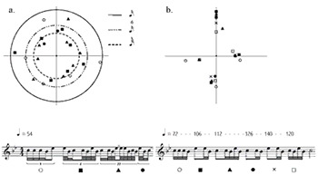
Figure 1. Microrhythmic morphing
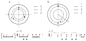
(click to enlarge)
[8] Figure 1a shows the tripletizing inflection discussed by Iyer (2002), in which a syncopated rhythm based on eighth- and sixteenth-notes is “spread” in order to accommodate a triplet-based grid.(3) Note value categories are shown as concentric circles.(4) The first (bracketed) pattern shows the quantized rhythmic template. As actually performed here, however, the durations are evened out through “spreading,” first mildly (first beat), then enough to transform the pattern into an isochronous triplet (second beat). The reverse type of microrhythmic morphing can be seen in Figure 1b, where the ternary long-short inflection is evened out to become a pair of even eighth-notes. On the second beat of the measure, the pattern closely resembles a triplet. The following two beats see a drive towards isochrony, such that the ternary long-short configuration is fully evened out by the beginning of the next measure. The diagonal gridline marks the beat’s two-thirds division—that is, where the eighth-note triplet (as shown in the transcription) would be aligned given a deadpan performance. Note that, unless marked with different point-shapes such as squares and triangles, the graph says nothing about which beat in the measure the notes belong to. It merely tracks cumulative onsets within the recursive tactus cycle. Neither does it presuppose a subdivision metric. Quite the opposite: all possible time-points in the beat are fair game; gridlines can be added after the fact to reveal any underlying metrical frameworks.
Analytical Contexts
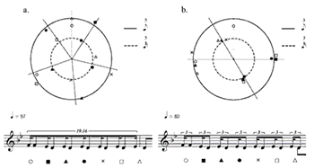
Figure 2. Bubber Miley (trumpet), “Creole Love Call”
(click to enlarge)
Figure 3. Wessell Anderson (alto saxophone), “Desimonae”
(click to enlarge)
Figure 4. Cumulative rhythmic activity across an 8-measure span
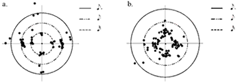
(click to enlarge)
[9] As shown, the circle graph can shed light on details of expressive timing. It can also prove useful in the analysis of rhythmically complex passages, such as the one shown in Figure 2a. The gridlines suggest that this rhythm may be organized according to a quintuplet grid. But, as the transcription shows, notating the rhythm accurately requires that we use a more complicated subdivision ratio (19:16) if the last note is to line up correctly with the downbeat of the next measure. Is there a grid that provides an alternative fit? Figure 2b suggests so. Even though the rhythm appears complex in its original tempo of 97 bpm, it can be rethought as a straightforward triplet pattern at 80 bpm—a tempo that may have momentarily supplanted the other one in the improviser’s mind. As Animation 3 shows, the ability to visually re-construe a given set of durations according to different clock speeds may constitute this graphing method’s biggest strength.
|
Animation 3
(click to view animation) |
Animation 4
(click to view animation) |
[10] Another potential purpose of the circle graph is to dissect nonperiodic rhythms that undergo a systematic retardation or acceleration. An example of such a rhythm appears in Figure 3. The transcription shows how each beat’s subdivision grid becomes successively finer as the notes get faster (6 to 8 to 10 subdivisions per beat; Figure 3a). Another way of interpreting the phrase is as a sixteenth-note grid that gradually contracts, as the alternate transcription shows (Figure 3b / Animation 4). In order to determine the precise nature of this tempo curve, we split the phrase into one-beat chunks (with one exception on the third beat) and, with the graph’s help, assign each segment a local tempo that provides a good visual fit. This graph is in fact a composite of six different superimposed graphs, each with its own tempo and set of coordinates according to formula (1).
[11] We need not restrict the circle graph to brief passages. Because the graph is essentially a round histogram, it can be used to provide a snapshot of overall rhythmic characteristics. Huron (2006, p. 178) did this with columned histograms to display onset frequency of occurrence for meter and hypermeter. Similarly, we can allow the circle graph to collapse rhythmic activity over longer time spans, as in the two 8-measure passages shown in Figure 4. Both are duets that feature an improvised string-instrument solo accompanied by a steady congas accompaniment (which is not graphed). At first sight, the graphs resemble an inexperienced marksperson’s target. But a moment’s reflection reveals rhythmic properties particular to each performance. Nelson González’s solo is heavily syncopated: his eighth-notes are almost always displaced (they fall on the second and fourth sixteenth-note “slots”), he rarely plays on the downbeat, and his use of successive dotted eighth-notes result in hemiolas (Figure 4a). By contrast, Jaco Pastorius uses sequences of sixteenth-notes to place equal stress on all four subdivisions (Figure 4b); there are indeed some syncopated eighth-notes but they are much less prominent than in the other solo. Pastorius’ rhythmic urgency is of a different kind: he encloses the bull’s-eye with rapid (sub-100 ms) sixteenth-note triplets, whereas the sixteenth-note accounts for González’s fastest value.
[12] That these observations may be gleaned from a standard transcription is immaterial. Of note is the graph’s capacity to display various aspects of timing concisely and simultaneously. In addition, the circle graph can be used to view, in the form of geometric rotation, temporal displacement of a rhythmic figure. For instance, a rhythm that is delayed or anticipated by a sixteenth-note results in a positive or negative 90-degree rotation. If the displacement is microrhythmic rather than metronomic, the shape will appear slightly rotated and mildly distorted.
[13] Finally, a word on some of the graph’s limitations. While useful in diverse contexts, this method’s reliance on a pattern of recurring and isochronous beats makes it an impractical choice for visualizing music that does not conform to this type of rhythmic organization. Even if a steady beat is present, it is not always easy or possible to determine its exact onset. Furthermore, the circle graph can neither relate expressive timing patterns to larger musical structures nor portray the detailed time course of a performance—these phenomena are best illustrated linearly.
Summary
[14] I have shown how the circle graph can serve diverse analytical functions. Its design facilitates understanding of beat subdivision details by making them apparent to the naked eye. Alternate tempos, either stable or fluctuating, can be sought visually to accommodate otherwise intractable rhythms. Lastly, the distribution pattern of points can summarize structural traits exhibited by different rhythmic patterns of any length from a few notes to a multi-measure performance.
Fernando Benadon
American University
Department of Performing Arts
4400 Massachusetts Avenue
NW Washington, D.C.20016
fernando@american.edu
Works Cited
Anku, W. (2000). “Circles and Time: A Theory of Structural Organization of Rhythm in African Music.” Music Theory Online 6(1).
Becker, J. (1980). Traditional Music in Modern Java: Gamelan in a Changing Society. Honolulu: The University Press of Hawaii.
Benadon, F. (2006). “Slicing the Beat: Jazz Eighth-notes as Expressive Microrhythm.” Ethnomusicology 50(1), 73–98.
Clarke, E. (1999). “Rhythm and Timing in Music.” In D. Deutsch (Ed.), The Psychology of Music. San Diego: Academic Press, 473–500.
Cohn, R. (2001). “Complex Hemiolas, Ski-hill Graphs and Metric Spaces.” Music Analysis 20(3), 295–326.
Collier, G. L., & Collier, J. L. (2002). “A Study of Timing in Two Louis Armstrong Solos.” Music Perception 19(3), 463–483.
Collins, J. (2004). African Musical Symbolism in Contemporary Perspective. Berlin: Pro Business.
Desain, P., & Honing, H. (2003). “The Formation of Rhythmic Categories and Metric Priming.” Perception 32(3), 341–365.
Foote, J., & Cooper, M. (2001). “Visualizing Musical Structure and Rhythm via Self-similarity.” Proceedings, International Conference on Computer Music (Habana, Cuba).
Friberg, A., & Sundberg, J. (1999). “Does Music Performance Allude to Locomotion? A Model of Final Ritardandi Derived from Measurements of Stopping Runners.” Journal of the Acoustical Society of America 105(3), 1469–1484.
Huron, D. (2006). Sweet Anticipation: Music and the Psychology of Expectation. Cambridge: MIT Press.
Iyer, V. (2002). “Embodied Mind, Situated Cognition, and Expressive Microtiming in African-American Music.” Music Perception 19(3):387–414
Lerdahl, F., & Jackendoff, R. (1983). A Generative Theory of Tonal Music. Cambridge: MIT Press.
Locke, D. (1996). “Africa/Ewe, Mande, Dagbamba, Shona, BaAka.” In Worlds of Music: An Introduction to the Music of the World’s Peoples, edited by Jeff Todd Titon. New York: Schirmer Books, 71–143.
London, J. (2004). Hearing in Time: Psychological Aspects of Musical Meter. New York: Oxford University Press.
McLachlan, N. (2000). “A Spatial Theory of Rhythmic Resolution.” Leonardo Music Journal 10, 61–67.
Palmer, C. (1996). “Anatomy of a Performance: Sources of Musical Expression.” Music Perception 13(3), 433–453.
Repp, B. H. (2002). “The Embodiment of Musical Structure: Effects of Musical Context on Sensorimotor Synchronization with Complex Timing Patterns.” In W. Prinz & B. Hommel (Eds.), Common Mechanisms in Perception and Action: Attention and Performance XIX. Oxford: Oxford University Press, 245–265.
Reynolds, R. (2004). “Compositional Strategies in ‘The Angel of Death’ for Piano, Chamber Orchestra, and Computer-processed Sound.” Music Perception 22(2), 173–205.
Shepard, R. (1983). “Demonstrations of Circular Components in Pitch.” Journal of the Audio Engineering Society 31, 641–649.
Todd, N. P. (1994). “The Auditory ‘Primal Sketch’: A Multiscale Model of Rhythmic Grouping.” Journal of New Music Research 23, 25–70.
Toussaint, G. (2005). “The Geometry of Musical Rhythm.” Proceedings, Japan Conference on Discrete and Computational Geometry (JCDCG 2004), 198–212.
Tymoczko, D. (2006). “The Geometry of Musical Chords.” Science 313, 72–74.
Wishart, T. (1996). On Sonic Art. Amsterdam: Harwood Academic Publishers.
Footnotes
1. I am grateful to Charles J. Limb, Bruno Repp and Henkjan Honing for their feedback on an earlier draft of this article.
Return to text
2. The “top” of the beat lies at the top of the circle. There are two logical alternatives to this configuration. The downbeat could lie at θ = 0 (equating the beginning of the beat with the beginning of the arc) or at θ = –π/2 (such that the
downbeat lies at the bottom of the circle and the upbeat at the top).
Return to text
3. The performance measurements used in the examples were
made by the author with the sound editor Peak 4. Measurement errors are
estimated to lie between ~5 and ~10 ms. All examples are drawn from improvised
music. When music notation appears below a graph, it is a transcription and not
a score.
Return to text
4. These are provided for visual reference only and have no bearing on the coordinate placement of points.
Return to text
Copyright Statement
Copyright © 2007 by the Society for Music Theory. All rights reserved.
[1] Copyrights for individual items published in Music Theory Online (MTO) are held by their authors. Items appearing in MTO may be saved and stored in electronic or paper form, and may be shared among individuals for purposes of scholarly research or discussion, but may not be republished in any form, electronic or print, without prior, written permission from the author(s), and advance notification of the editors of MTO.
[2] Any redistributed form of items published in MTO must include the following information in a form appropriate to the medium in which the items are to appear:
This item appeared in Music Theory Online in Volume 13, Issue 3 in September 2007. It was authored by Fernando Benadon (fernando@american.edu), with whose written permission it is reprinted here.
[3] Libraries may archive issues of MTO in electronic or paper form for public access so long as each issue is stored in its entirety, and no access fee is charged. Exceptions to these requirements must be approved in writing by the editors of MTO, who will act in accordance with the decisions of the Society for Music Theory.
This document and all portions thereof are protected by U.S. and international copyright laws. Material contained herein may be copied and/or distributed for research purposes only.

Prepared by Brent Yorgason, Managing Editor and Stefanie Acevedo, Editorial Assistant
Number of visits: