Solutions to the “Great Nineteenth-Century Rhythm Problem” in Horowitz’s Recording of the Theme from Schumann’s Kreisleriana, Op. 16, No. 2
Alan Dodson
KEYWORDS: microtiming, phrase rhythm, meter, Schumann, Horowitz
ABSTRACT: This case study on the interpretation of microtiming is framed by the hypothesis that the avoidance of monotony in the case of highly regular phrase/hypermetric structures was not only one of the great compositional problems of the nineteenth century, as William Rothstein has proposed, but also was and remains a problem for performers. This analytical strategy helps to organize and synthesize diverse observations about a complex set of subtle microtiming practices in the titular recording. It is shown that Horowitz introduces subtle variations when materials are repeated, and that he tends to bring out the most salient aspects of Schumann’s own solutions to the “rhythm problem” (metric tensions, contrasts in rhythmic shape), except in cases of phrase linkage. This study suggests that principles of phrase rhythm could make a valuable contribution to the analytical toolbox for performance studies.
Copyright © 2012 Society for Music Theory
[1] The empirical and statistical tools that music theorists interested in performance have borrowed from our colleagues in other disciplines (see Clarke 2004) offer considerable clarity and precision, and these tools will no doubt continue to evolve in the years ahead. Even at its most precise, however, the analysis of microtiming data tends to produce results that are heterogeneous and resistant to interpretation, and we are still at the stage where new analytical strategies need to be developed and evaluated. In the present study, I am especially interested in exploring ways in which a familiar, speculative (theoretically driven) approach to the analysis of works can feed into the lexicon for the interpretation of microtiming.(1) At the outset I think it is important to mention that although the object of my analysis—the microtiming in a recording—was measured in a very precise way, my interpretation of that object is by no means “scientific” or “objective.” As Marion Guck has demonstrated, “musical analyses typically—necessarily—tell stories of the analyst’s involvement with the work she or he analyzes” (Guck 1994, 218). Accordingly, this case study should be taken as only one of many possible readings of the microtiming in a recording.
[2] In Phrase Rhythm in Tonal Music, William Rothstein points out that a “danger...of too unrelievably duple a hypermetrical pattern, of too consistent and unvarying a phrase structure” was “endemic in nineteenth-century music,” and he refers to this danger, memorably, as the “Great Nineteenth-Century Rhythm Problem” (GNCRP) (Rothstein 1989, 184–85). Rothstein makes frequent reference to the GNCRP in the analytical chapters that comprise the second part of his book. He shows that Romantic-era composers did not necessarily have to retreat to an earlier, more elastic style in order to solve the GNCRP, although some (most notably Mendelssohn) did so. For other composers, such as Chopin and Wagner, the solution to the GNCRP lay not so much in manipulating the phrase lengths as in finding new ways to conceal—and ultimately to transcend—phrase boundaries and thereby to achieve the effect Wagner referred to as “endless melody.” These composers, in other words, solved the GNCRP not by avoiding regular metric and grouping structures, but instead by enlivening them in novel ways so that their effect would not become mechanical and tiresome.
[3] I would like to build on Rothstein’s composer-centered narrative by proposing that the GNCRP was a problem not only for composers, but also for performers. This problem can be solved by performers, I suggest, through effective use of the various expressive means under their control, including subtleties of microtiming. I will try to demonstrate this through a short case study on both the composer’s and the performer’s solutions to the GNCRP in a recording by Vladimir Horowitz of the theme from the second movement of Schumann’s Kreisleriana, op. 16 (“Sehr innig und nicht zu rasch”) (Horowitz 2011, first issued 1969).(2) Some readers will find it self-evident that the manner of performance can mitigate the risk of musical monotony, a danger that is especially acute in the case of works that feature a high level of rhythmic regularity. However, the ramifications of this idea have not yet been explored in the theoretical literature on phrase rhythm or in the empirical literature on microtiming, so a case study seems warranted.
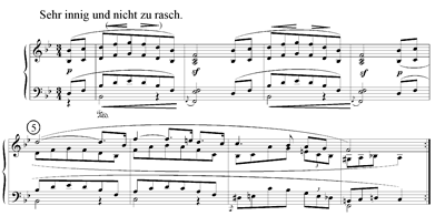
Example 1. Schumann, Kreisleriana, op. 16, no. 2, theme
(click to enlarge and see the rest)
[4] The score, based on the version in the Gesamtausgabe edited by Clara Schumann (Schumann 1887) is provided as Example 1. The rhythmic structure of the theme is very regular; duple hypermeter and four-bar grouping (with one-beat anacrusis) are present throughout, and there are continuous eighth-note subdivisions in all but six of the theme’s thirty-seven measures. Overall, the work has a clear rounded binary form with coda, within which the four-bar groups combine to form three phrases of ever-increasing length:
- A (measures 1–8, repeated)
- B (measures 9–20)
- A’ (measures 21–28) + coda (measures 29–37)
Each of these phrases is supported by a straightforward harmonic progression: I–![]() –IV5–6–VI–(II–VI)– II
–IV5–6–VI–(II–VI)– II![]() –V (measures 9–20), I–
–V (measures 9–20), I–
[5] The high degree of variability in the microtiming of Horowitz’s recording presents us with an abundance of information to interpret. I provide two short excerpts from it here (Example 4 below); I encourage readers to listen to the entire recording, which is widely available at university music libraries and can also be purchased from various online vendors, including iTunes and Amazon.com.
[6] I studied the recording using Sonic Visualiser, a program designed by researchers affiliated with the Centre for the History and Analysis of Recorded Music (Cook and Leech-Wilkinson 2009).(3) I began by listening to the recording repeatedly at the normal playback speed and taking note of the most salient expressive details, including many examples of tempo variation and asynchrony. By “tempo variation,” I mean a momentary change in speed and/or quality of motion, and by “asynchrony,” I mean grace notes (which have no specified metrical position) as well as situations in which notes that occupy the same metrical position are executed in a non-simultaneous fashion, namely hand displacements (where the left hand plays marginally before or after the right) and arpeggiations.
[7] I sharpened and refined these preliminary observations through empirical analysis. To track the tempo variations, I first used a tool in Sonic Visualiser that records the counter times of each keystroke as I tapped along with the recording, with playback speed reduced by 50%. Next, I used a tool that automatically identifies the physical onset time of each note in the recording,(4) followed by a tool that selects the physical onset that falls closest to each of my tap times.(5) Finally I made corrections, as needed, using a click track and spectrogram as guides. To make the measurements as accurate as possible, I gradually reduced the playback window to find the cusp at which each event becomes audible, which in every case corresponded to a clear discontinuity in the spectrogram. Making corrections in this way is time-consuming, but it is thought to be the most accurate approach to microtiming analysis. The three-step procedure that I have outlined—tapping, automated onset detection and alignment, and manual correction—is among the most efficient and accurate procedures currently available for the analysis of tempo variations; it combines the advantages of two earlier approaches (one based on tapping, the other on manual onset detection, see Clarke 2004) while mitigating their disadvantages. I used this method to identify all of the note onsets in the recording at the eighth-note level. Subtracting the onset times of successive beats at a given level yields a series of durations. Based on these calculations, I prepared tempo graphs at both the quarter-note (tactus) and eighth-note level. I then measured the asynchronies that were audible at full playback speed by locating the onsets of the relevant events, again using the spectrogram tool in Sonic Visualiser. For arpeggiations, I measured the time between the first and last onsets (i.e., between the bass note and the melody note).(6) For all asynchronies, I used the melody note for purposes of tempo tracking, as is customary in the empirical literature.
[8] Results of the empirical analysis are shown in Examples 4–6, 8–10, 12–13, and 15–16. In each case, the upper graph shows durations at the quarter-note (tactus) level, while the lower graph shows durations at the eighth-note level. Readers unfamiliar with these kinds of graphs may find it helpful to think of a mechanical metronome: the higher a data point’s position on the page, the slower the tempo. A few tactus pulses are unarticulated (e.g., measure 2.2), and in these cases the durations of two successive timespans—those for which the unarticulated pulse serves as endpoint and starting-point—cannot be measured using the method employed in this study.(7) Accordingly, in such instances there are gaps in the graph. Asterisks above the score indicate asynchronies, only some of which are indicated in the score through arpeggiation signs or grace notes. In each case, the discrepancy (in milliseconds) between the first and last onset times is provided.
[9] My illustrations of the microtiming in Horowitz’s recording will take the form of line graphs. Although this format displays the essential information clearly, it does have at least one counterintuitive and potentially confusing feature: the line segments between the data markers might, at first glance, be taken to represent continuous tempo change during the timespan in question—that is, one might assume that an ascending or a descending slope indicates that a tempo change is already underway before the next beat is articulated. This would be a false assumption, because each data marker represents the duration of a metric event. Thus, for instance, descending slope over a barline indicates that the upbeat is longer than the downbeat, not that there is an acceleration from the upbeat to the downbeat. Indeed, if there were such an acceleration then the upbeat would in consequence be shortened, not lengthened. In other words, these graphs represent tempo change as an articulated phenomenon, not a continuous one. Beat-to-beat tempo changes are represented by the relative position of the data markers, but instant-to-instant tempo changes are not represented by the slope of the line segments between them.(8)
[10] As with any empirical approach, the limitations of the tools must be acknowledged. Some measurement error is inevitable because of occasional buzzing or other noise around the time of an onset. There are probably individual differences in how listeners entrain to the music, particularly in phrases that have asynchronies; some listeners may entrain to the first event (e.g., the bottom note of an arpeggiated chord), others to the last event (the top note), and some may experience a blurring of the beat when asynchronies are used (see Yorgason 2009). Most importantly, some tempo changes are too small to be audible; the threshold seems to fall somewhere in the range of 10 to 40 ms (Benadon 2007, [15]), and it appears to be proportional to the basic tempo (Halpern and Darwin 1982). The salience of a tempo change is also affected by its grouping context; tempo changes that adhere to stylistic norms (e.g., deceleration at the end of a phrase) tend to be less noticeable than those that diverge from the norm (Repp 1998). Finally, the contour of the tempo graph does not always give a clear reflection of the qualities of motion that the listener experiences. Beyond the possible confusion arising from the line segments between the data markers (discussed above), it should be noted that some aurally distinct phenomena (e.g., hesitation, tenuto, and ritardando) are indistinguishable from each other on the basis of a tempo graph alone, a point that is seldom acknowledged in the empirical literature (but see Dodson 2002, [3.5] and passim). In an effort to compensate for this limitation, I have added annotations that describe the aural effects of many details, as I experience them. Despite their outwardly scientific appearance, then, such graphs are partly based on personal, subjective judgments. They can nevertheless be valuable in guiding and sharpening the reader’s listening experience, so I will refer to them often in the discussion that follows.
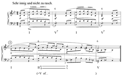
Example 2. Schumann, Kreisleriana, op. 16, no. 2, annotated score of measures 1–8
(click to enlarge)
[11] Before turning to details in the recording, it will be useful to consider Schumann’s solution to the GNCRP in the opening phrase (measures 1–8, see Example 2), and in particular to consider how he uses metrical tension to provide the phrase with inner vitality and shape. The harmony and grouping provide a basic orientation for duple hypermeter from the outset, but phenomenal accents in measures 2 and 4 (i.e., harmonic dissonance, durational accents, dynamic accents, and density accents) project a displacement of that hypermeter strongly. There is, in other words, a conflict between the basic hypermeter and another six-beat periodicity that serves as its “shadow” (to borrow a metaphor from Samarotto 1999).(9) Using Krebs’s labeling system for displacement dissonance, where the first number indicates the periodicity and the second indicates the size of the displacement (Krebs 1999, 35), this situation can be represented as D6+3 (1 = quarter note). These periodicities are labeled within and above the score in Example 2, and in similar examples below, while a harmonic analysis is given below the score. The tension between the hypermeter and its shadow continues in the second half of the phrase. Here the grouping structure leaves no doubt as to the primacy of the odd-strong hypermeter, but the registral accent (F5) and harmonic dissonance (![]()
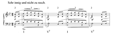
Example 3. Schumann, Kreisleriana, op. 16, no. 2, annotated score of measures 1–4
(click to enlarge)
[12] In addition to the three- and six-beat metrical layers, a two-beat layer is established in the first half of the phrase through the registral and dynamic accents at measure 1.2 and the various phenomenal accents at measure 2.1 (see Example 3). In retrospect, this duple layer is understood to begin at the first note of the melody. The progression in accentual force from each beat of this layer to the next gives it something of the character of an extended anacrusis—one that culminates, notably, at the point at which the duple layer and the hypermeter’s shadow converge. The conflict between the duple layer and the primary layer (the notated meter) involves both displacement and metric grouping, so it is an example of what Krebs calls a compound metrical dissonance (Krebs 1999, 59–60). Overall, the rhythm of this opening phrase is far from being mechanical and predictable, despite its clear, regular hypermeter. The metrical dissonances I have mentioned enliven it with inner tension and momentum.
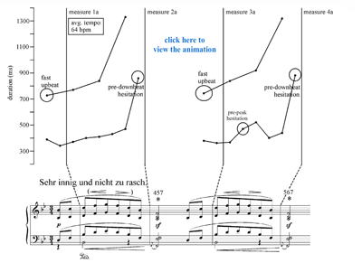
Example 4. Schumann/Horowitz, Kreisleriana, op. 16, no. 2, measures 1–8a
(click to open the animation)
[13] Example 4 is an animation that shows the microtiming in the first eight measures from Horowitz’s recording. One of the first things one notices in the recording is that whereas Schumann’s expression markings draw attention to the even-numbered downbeats (the “shadow”), Horowitz instead concentrates on reinforcing the odd-numbered downbeats. Indeed, he all but ignores the crescendo and sf markings in measures 1–4, and he adds a strong dynamic accent at the downbeat of measure 5. In the first half of the phrase, he emphasizes the odd-numbered downbeats mainly by playing the beats that precede them relatively quickly. This inherently increases the upbeats’ anacrustic quality (Butterfield 2006, also Hasty 1997, 164). In contrast to his handling of the first and third downbeats, he hesitates very noticeably before the downbeats of measures 2 and 4, thereby allowing the anacrustic energy to dissipate somewhat. He also hesitates slightly before the melodic peaks at measures 1.2 (second time only, see Example 5) and 3.2 (both times), thereby highlighting the point in the melodic gesture where the duple layer comes into focus. Although Horowitz’s reading of the phrase is far from literal, it arguably does enhance the metric tension latent within the music. As Krebs has pointed out, in the case of metrically dissonant passages, the primary metrical layer is often less salient than the competing layers, and in such cases emphasizing the primary layer can be an effective performance strategy (Krebs 1999, 179). It is possible, then, to read Horowitz’s solution to the GNCRP as an extension of Schumann’s own.
|
Example 5. Schumann/Horowitz, Kreisleriana, op. 16, no. 2, measures 1–4b
(click to enlarge) |
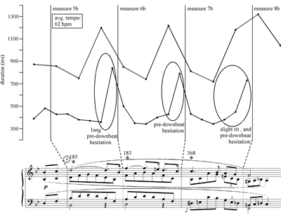
Example 6. Schumann/Horowitz, Kreisleriana, op. 16, no. 2, measures 5–8b
(click to enlarge) |

[14] There is more to Horowitz’s solution than this, however. By introducing subtle variations in the second iteration of the phrase, he enlivens the music in ways that have no parallel in the score. One subtle difference is that in the first half of the phrase, he displaces the bass notes by a full eighth-note during the first iteration but plays them decisively on the beat the second time through. Another difference is that there are more asynchronies the second time (compare Example 4 to Examples 5–6); on the first iteration Horowitz adds only one salient asynchrony, at measure 7.1, beyond the two indicated in the score through grace notes (at measures 2.1 and 4.1), but on the second iteration he adds further asynchronies at the downbeats of measures 3, 5, and 6. A third difference is that although he hesitates before measures 1.2 and 3.2 both times, the delay is longer the second time through (average delay: 65 ms first time, 105 ms second time). Similarly, his pre-downbeat hesitations are in most cases longer the second time through. The difference is especially pronounced in the second half of the phrase; the average delay is 240 ms the first time and 375 ms the second time, and the longest hesitation of all (480 ms) sets off the second iteration of measure 6.1, the point where the hypermeter’s shadow begins to recede. In all of these ways, Horowitz subtly reinforces many of the conflicting metric accents during the repetition of the phrase, including those associated with the bar meter, the hypermeter and its shadow, and the duple layer at the beginning of the phrase. Thus, his handling of the repeat not only lends his performance a subtle improvisatory quality that itself helps to sustain the listener’s attention, but also draws that attention more forcefully to musical elements that relate, in some way, to the metrical innovations that lie at the core of Schumann’s own solution to the GNCRP in this phrase.
Example 7. Schumann, Kreisleriana, op. 16, no. 2, annotated score of measures 9–20

(click to enlarge and see the rest)
[15] In the second phrase (measures 9–20, Example 7), Schumann solves the GNCRP by giving each four-bar subphrase a distinct rhythmic shape. In the first subphrase (measures 9–12), the melody (now in the left hand) ascends gradually to ![]() –IV, II
–IV, II![]() –V) while the second has purely consonant, triadic harmony and plagal motion;(10) the first subphrase has melodic activity in the left hand, the second in the right hand, and the third in both hands (see the countermelody in the tenor); the melody ascends in the first subphrase, descends in the second, and moves in an arch shape in the third; and the counterpoint emphasizes oblique motion in the first subphrase (see the static descant), similar motion in the second, and contrary motion in the third. In all of these respects, contrast lies at the heart of Schumann’s solution to the GNCRP within the second phrase.(11)
–V) while the second has purely consonant, triadic harmony and plagal motion;(10) the first subphrase has melodic activity in the left hand, the second in the right hand, and the third in both hands (see the countermelody in the tenor); the melody ascends in the first subphrase, descends in the second, and moves in an arch shape in the third; and the counterpoint emphasizes oblique motion in the first subphrase (see the static descant), similar motion in the second, and contrary motion in the third. In all of these respects, contrast lies at the heart of Schumann’s solution to the GNCRP within the second phrase.(11)
Example 8. Schumann/Horowitz, Kreisleriana, op. 16, no. 2, measures 9–12
(click to enlarge)
Example 9. Schumann/Horowitz, Kreisleriana, op. 16, no. 2, measures 13–16
(click to enlarge)
Example 10. Schumann/Horowitz, Kreisleriana, op. 16, no. 2, measures 17–20
(click to enlarge)
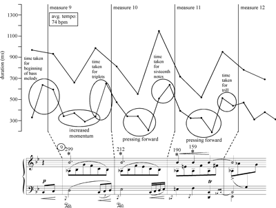
[16] Horowitz emphasizes many of these contrasts, and his microtiming underscores each subphrase’s distinct quality of motion. In the first subphrase (Example 8), his average tempo (809 ms, equivalent to 74 beats per minute) is considerably faster than in the work’s opening phrase (62 bpm overall), and this tempo change reinforces the dynamic and teleological character of this subphrase. Within each measure, Horowitz accelerates through the second beat and draws out the first and third beats, so that the ascending left-hand melody and the progression of rhythmic values can be heard clearly. This results in a V-shaped tempo profile within each measure. Horowitz’s interpretation of Schumann’s grace notes is also noteworthy; his asynchronies become gradually shorter as the subphrase proceeds, and this conveys a sense of motion towards a goal, namely the point of zero asynchrony at the downbeat of measure 12. Paradoxically, the very lack of an asynchrony at that point gives it a strong sense of arrival and emphasis.(12)
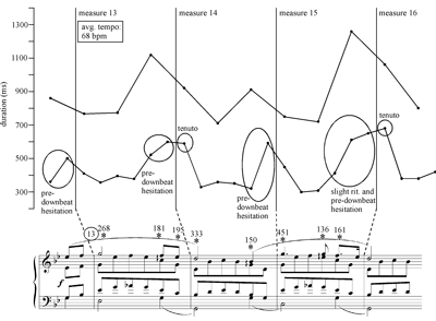
[17] In keeping with the second subphrase’s more relaxed character, Horowitz plays it at a somewhat slower tempo (68 bpm) and adds a total of eight gentle asynchronies, only two of which are indicated in the score (Example 9). The greatest of these asynchronies (333 ms) falls on the downbeat of measure 15 and conveys a subtle sense of intensification at the registral peak of the second two-bar gesture. Horowitz sets off all four downbeats by hesitating slightly before them and by lengthening the first eighth note in each measure slightly; this gives the subphrase a poised, unhurried quality that differs markedly from the musical effect of measures 9–12.
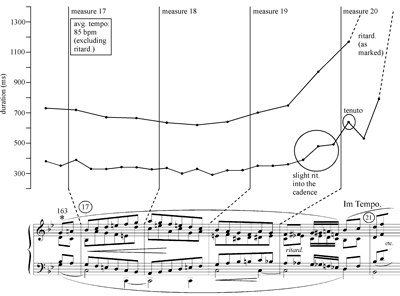
[18] In the third subphrase (Example 10), Horowitz takes an even faster average tempo than in the first (84 bpm, excluding the ritard), and he abandons the V-shaped tempo profile within the measure—a pattern evident in both of the preceding subphrases—in favor of a single tempo arch spanning the entire subphrase. Through inspection of the lower graph, it is also evident that the durations of his eighth notes are much more consistent here than elsewhere in the piece; it is here that Horowitz’s capacity for rhythmic precision and control is demonstrated most clearly. Another notable feature of this subphrase is that the parts are tightly coordinated throughout; there is only one audible asynchrony here, located at the very beginning of the subphrase (at measure 16.3). Taken together, these features give measures 17–20 a stronger sense of continuity and momentum than any other unit in the piece.
[19] Schumann employs an innovative combination of phrase linkage techniques in measure 20, at the boundary of the theme’s second and third phrases. As mentioned above, the bass note (F) is withheld at the downbeat of measure 20, where the cadence point is reached. The result is an unstable ![]()
![]()
[20] Horowitz does surprisingly little to emphasize the tensions inherent in measure 20. He signals the arrival of the cadence by adding a slight ritard toward the end of measure 19, followed by an elongation (tenuto accent) at the cadence point itself (measure 20.1). He makes much of the prescribed ritard in beats 1–2 of measure 20, where the tempo profile goes off the scale, but it sounds as though he ignores the continuation of the left-hand slur to beat 3 and the sense of continuity that it implies. This situation could perhaps be read as a decision on Horowitz’s part that bringing out the instability in measure 20 (for instance, by emphasizing the bass C and D and making a legatissimo connection between these notes) would sound overwrought or otherwise unpleasing. Aesthetic judgment is, after all, an essential part of interpretation, and for this reason only some subtleties are brought out by performers, while others are left alone.
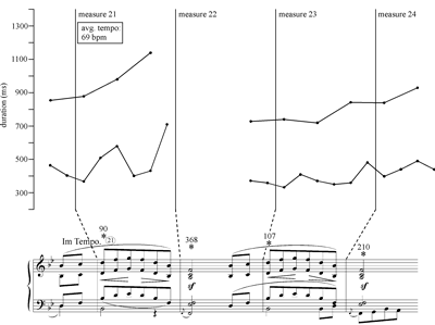
Example 11. Schumann, Kreisleriana, op. 16, no. 2, annotated score of measures 21–28

(click to enlarge)
Example 12. Schumann/Horowitz, Kreisleriana, op. 16, no. 2, measures 21–24
(click to enlarge)
Example 13. Schumann/Horowitz, Kreisleriana, op. 16, no. 2, measures 25–28
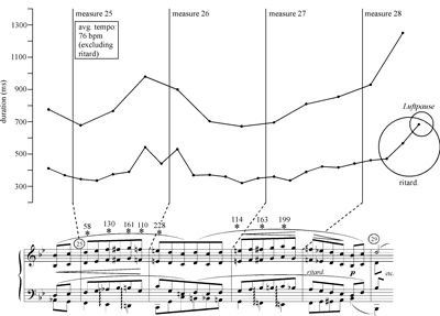
(click to enlarge)
[21] The third phrase (measures 21–28) begins with a nearly literal return of material from measures 1–4 (Example 11). The first significant change occurs in measure 24, where a new bass gesture provides added momentum into the material that follows in measures 25–28—material that differs radically from measures 5–8 in ways that add further complexity to the metrical structure. Crescendo markings now point toward the downbeats of measures 26 and 28, thereby reinforcing the hypermeter’s shadow instead of allowing it to recede in the second half of the phrase. Melodic peaks in measures 25 and 27 now precede the shadow by one beat in each case, so that for the first and only time in the theme there are three distinct six-beat periodicities: the hypermetric layer (projected by the odd-numbered downbeats), its shadow (projected by the even-numbered downbeats), and a displacement of the shadow (projected by the registral accents at measures 25.3 and 27.3). The theme’s surface-level harmonic instability also reaches its high point here (see especially the ![]()
[22] Horowitz highlights these changes in a number of ways (Examples 12–13). First of all, he takes a faster basic tempo than before (72 bpm in measures 21–28 [excluding the ritard], compared to 62 bpm in measures 1–8), and he brings out the new bass figure in measure 24 simply by playing it louder (not through microtiming). On a more subtle level, he adds small asynchronies at the downbeats of measures 21 and 23, and the alternation between these and the larger asynchronies at the downbeats of measures 22 and 24 underscores the metrical dissonance. As seen in Example 13, he adds eight further asynchronies in measures 25–28, only four of which are prescribed in the score. Three of his extra asynchronies fall on downbeats, and these once again project a short-long-short pattern that reinforces the metrical dissonance in a subtle way. The remaining asynchrony (found at the end of measure 25), like the four that are indicated in the score, occurs during a crescendo that projects the D6+3 pattern. Also noteworthy is the relatively high degree of continuity in Horowitz’s performance of this passage, especially in measures 26–27, where a single harmony (
[23] One challenging point in the analysis of the theme’s form concerns the third phrase’s cadence. (For the broader musical context, see again Example 1.) Is there a half cadence at measure 28.1, followed by a lead-in to the coda, or is there an authentic cadence at measure 29.1 (or perhaps measure 28.3), with a phrase overlap? If these were the only options, then I would choose the first option for at least two reasons: the bass ascends by step from to in measure 28, a gesture much more characteristic of a lead-in than a cadence, and measures 28.3–29.1 initiate the reprise, so these beats sound much more like a beginning than an ending. This half-cadence reading is not entirely satisfying, however. Its main shortcoming is that it suggests that the tonic chords at measures 28.3 and 29.1, and also the ensuing tonic prolongation in measures 29–37, are entirely separate from the cadential process and, therefore, that the theme as a whole (measures 1–37) essentially ends with a structural half cadence at measure 28.1. (The coda has a pedal bass throughout, so there is no possibility of an authentic cadence after measure 28. Although there is a clear V–I motion in measures 36.3–37.1, even this cannot be regarded as the structural cadence, because a prolongation of the final tonic is established long before this point.) As Poundie Burstein has recently proposed, complex situations like the one found in measure 28 highlight inadequacy of a binary (“black-and-white”) conception of cadence types in tonal music and point to the need for additional categories along a spectrum of cadential possibilities (Burstein 2010). The absence of an “Im Tempo” marking after the ritard in measure 28 enhances the ambiguity somewhat; the ritard heightens the sense of “ending” associated with the cadence, and the return to the main tempo heightens the sense of beginning, but the lack of an “Im Tempo” means that we cannot tell, based on the tempo markings in the score alone, precisely where the feeling of ending ends, where the sense of beginning begins, and whether there is any transitional zone between these diametrically opposed qualities of motion. In this case, the rhythmic and metric aspects of the cadence suggest that it lies closer to the “half cadence” pole of Burstein’s spectrum, while the stylistic conventions associated with the form, and with tonal music in general, push it a few notches in the direction of the “authentic cadence” pole. Regardless of how we decide to interpret the cadence type, its ambiguity (from the vantage of conventional conceptions of cadence) complicates the grouping boundary by blending aspects of continuity and discontinuity, so this can be understood as a further example of linkage technique.(13)
Audio Example 1. Vladimir Horowitz
Audio Example 2. Walter Gieseking
Audio Example 3. Murray Perahia
Example 14. Schumann, Kreisleriana, op. 16, no. 2, annotated score of measures 29–37
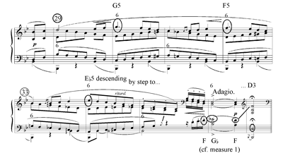
(click to enlarge)
[24] Amid the play of opposing forces in measure 28, Horowitz once again tips the scales in favor of discontinuity, just as he had done in measure 20. He makes much of the ritard in measure 28.1–28.2 and adds a Luftpause after measure 28.2 (see again Example 13) before returning to the main tempo at measure 28.3. He also makes a clear dynamic contrast (to f, not p as marked) at measure 28.3 (Audio Example 1).These details seem to push measure 28 almost entirely toward the “half cadence” pole. As in the case of measure 20, Horowitz does nothing to highlight the tensions inherent in the linkage. It would be premature to suggest on the basis of just two examples that this represents a basic feature of his performing style (a general aesthetic preference), but perhaps this is a topic worthy of further study. A close comparison to other recordings is also revealing; some other performers, such as Walter Gieseking (Audio Example 2) and Murray Perahia (Audio Example 3), convey a clear sense of continuity into the coda, in terms of both rhythm and dynamics—continuity that traverses the grouping boundary and pushes the effect toward the “authentic cadence” pole.
[25] Harmonic motion ceases once the tonic harmony is reached; as noted above, a pedal bass is present throughout the coda, which lasts from measure 29 until the end of the theme (Example 14). Despite this harmonic stasis, within the coda a sense of directed motion is conveyed through a descent from the registral peaks G5 (measure 30), F5 (measure 32), and
Example 15. Schumann/Horowitz, Kreisleriana, op. 16, no. 2, measures 29–32
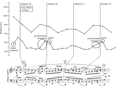
(click to enlarge)
Example 16. Schumann/Horowitz, Kreisleriana, op. 16, no. 2, measures 33–37
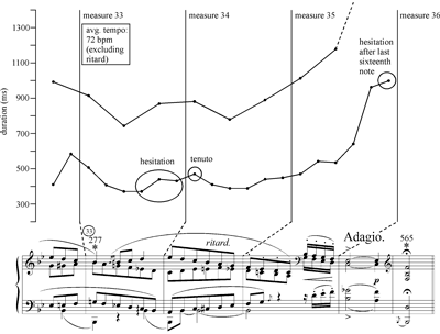
(click to enlarge)
[26] Horowitz brings out the metric tensions in the coda not so much by reinforcing the main hypermetric layer as by supplying dynamic accents for the melodic peaks that project its shadow. He does, however, bring out the main hypermeter subtly by making much of the asynchronies that are necessitated by the wide spacing in the left hand in most of the odd-numbered measures of the coda (see Examples 15–16). In short, he uses dynamic accents to make one of the six-beat layers conspicuous, and he uses microtiming to draw more subtle attention to the other.
[27] This preliminary study supports the hypothesis that the GNCRP was a problem not only for composers but also for performers and suggests that it can provide a useful focal point in the interpretation of recordings. In the theme we have been examining, Schumann solves the GNCRP by enlivening phrases through metrical tension and directed harmonic/linear motion, and through contrasts in texture and harmonic rhythm between successive subphrases. Beyond the phrase level, he sustains musical tension through linkage techniques and, it might be added, by developing the F5–G5–F5 motive in a variety of subtle ways. (The chromaticized version in measure 36, mentioned above in paragraph 25, is only the most conspicuous variation. For a comprehensive account of the many guises of the F5–G5–F5 motive throughout the movement, see Fisk 1997.) Horowitz, in turn, solves GNCRP partly by bringing out aspects of Schumann’s own solutions (the metric tensions and qualitative contrasts in rhythm), and partly by introducing subtle variations in the repeated materials. He is highly selective; in particular, he makes no attempt to underscore the linkage techniques, and in the case of metric conflicts he often simply reinforces the primary metric layer and the hypermetric (odd-strong) layer.
[28] Further research would be needed in order to determine the scope of the GNCRP’s relevance to the interpretive practices of performers of the past and present, but on the basis of the present study it seems that the GNCRP and other principles of phrase rhythm could make a valuable contribution to the toolbox for performance analysis. This kind of approach is far from being objective, and those who favor a more scientific approach may think that it borders on overinterpretation. For those who can suspend disbelief, however, phrase rhythm could perhaps be a focal point in a sustained study of a given performer’s style, or in a comparison of different recordings of a given work. This is just one of the many ways in which music theory might make a distinctive and valuable contribution to the analysis and interpretation of recordings, a field of study that is now beginning to rise above its necessarily positivistic and empirical roots through the participation of scholars from a wide variety of disciplines.
Alan Dodson
University of British Columbia
School of Music
Vancouver, BC Canada V6T 1Z2
alan.dodson@ubc.ca
Works Cited
Benadon, Fernando. 2007. “Commentary on Matthew W. Butterfield’s ‘The Power of Anacrusis’.” Music Theory Online 13, no. 1. http://www.mtosmt.org/issues/mto.07.13.1/mto.07.13.1.benadon.html
Burstein, L. Poundie. 2010. “Half, Full, or In Between? Distinguishing Half and Authentic Cadences.” Annual Meeting of the Society for Music Theory. Indianapolis, IN, 6 November.
Butterfield, Matthew W. 2006. “The Power of Anacrusis: Engendered Feeling in Groove-Based Musics.” Music Theory Online 12, no. 4. http://www.mtosmt.org/issues/mto.06.12.4/mto.06.12.4.butterfield.html
—————. 2011. “Why Do Jazz Musicians Swing Their Eighth Notes?” Music Theory Spectrum 33, no. 1: 3–26.
Caplin, William E. 1998. Classical Form: A Theory of Formal Functions for the Instrumental Music of Haydn, Mozart, and Beethoven. New York: Oxford University Press.
Carey, Norman. 2007. “An Improbable Intertwining: An Analysis of Schumann’s Kreisleriana I and II, with Recommendations for Piano Practice.” Theory and Practice 32: 19–50.
Clarke, Eric F. 2004. “Empirical Methods in the Study of Performance.” In Empirical Musicology: Aims, Methods, Prospects, ed. Eric F. Clarke and Nicholas Cook, 77–102. New York: Oxford University Press.
Cook, Nicholas, and Daniel Leech-Wilkinson. 2009. “A Musicologist’s Guide to Sonic Visualiser.” London: Centre for the History and Analysis of Recorded Music. http://www.charm.rhul.ac.uk/analysing/p9_1.html (accessed August 11, 2011).
Cooper, Grosvenor, and Leonard B. Meyer. 1960. The Rhythmic Structure of Music. Chicago: The University of Chicago Press.
Dixon, Simon. 2001. “Automatic Extraction of Tempo and Beat from Expressive Performances.” Journal of New Music Research 30: 39–58.
Dodson, Alan. 2002. “Performance and Hypermetric Transformation: An Extension of the Lerdahl-Jackendoff Theory.” Music Theory Online 8, no. 1. http://www.mtosmt.org/issues/mto.02.8.1/mto.02.8.1.dodson_frames.html
—————. 2008. “Performance, Grouping and Schenkerian Alternative Readings in Some Passages from Beethoven’s ‘Lebewohl’ Sonata.” Music Analysis 27, no. 1: 107–34.
—————. 2009. “Metrical Dissonance and Directed Motion in Paderewski’s Recordings of Chopin’s Mazurkas.” Journal of Music Theory 53, no. 1: 57–94.
Fisk, Charles. 1997. “Performance, Analysis, and Musical Imagining Part II: Schumann’s Kreisleriana, No. 2.” College Music Symposium 37: 95–108.
Gabrielsson, Alf. 2003. “Music Performance Research at the Millenium.” Psychology of Music 31, no. 3: 221–72.
Guck, Marion. 1994. “Analytical Fictions.” Music Theory Spectrum 16, no. 2: 217–30.
Halpern, Andrea R., and Christopher I. Darwin. 1982. “Duration Discrimination in a Series of Rhythmic Events.” Perception and Psychophysics 31, no. 1: 86–89.
Hasty, Christopher. 1997. Meter as Rhythm. New York: Oxford University Press.
Horowitz, Vladimir. 2011. Schumann: Kreisleriana, op. 16, Wieck-Variations, Kinderszenen, op. 15, Toccata in C Major, op. 7. Recorded 1969. Issued Sony Classical 7858312. Compact disc.
Krebs, Harald. 1999. Fantasy Pieces: Metrical Dissonance in the Music of Robert Schumann. New York: Oxford University Press.
Lerdahl, Fred, and Ray Jackendoff. 1983. A Generative Theory of Tonal Music. Cambridge, MA: MIT Press.
London, Justin. 2004. Hearing in Time: Psychological Aspects of Musical Meter. New York: Oxford University Press.
Perahia, Murray. 1997. Schumann: Kreisleriana, Piano Sonata No. 1. Recorded 1997. Issued Sony Classical 62768.
Repp, Bruno H. 1998. “The Detectability of Local Deviations from a Typical Expressive Timing Pattern.” Music Perception 15, no. 3: 265–90.
Rothstein, William. 1989. Phrase Rhythm in Tonal Music. New York: G. Schirmer.
Samarotto, Frank. 1999. “Strange Dimensions: Regularity and Irregularity in Deep Levels of Rhythmic Reductions.” In Schenker Studies 2, ed. Carl Schachter and Hedi Siegel, 222–38. New York: Cambridge University Press.
Schumann, Robert. 1887. Kreisleriana, op. 16 (composed 1838, revised 1848). Robert Schumann’s Werke, ed. Clara Schumann, Serie VII: Für Pianoforte zu zwei Händen. Leipzig: Breitkopf & Härtel.
Yorgason, Brent. 2009. “Expressive Asynchony and Meter: A Study of Dispersal, Downbeat Space, and Metric Drift.” Ph.D. diss., Indiana University.
Footnotes
1. In this sense, the study builds on other recent scholarship on microtiming that engages and adapts pre-existing theories of compositional structure (e.g., Butterfield 2006, 2011; Dodson 2002, 2008, 2009).
Return to text
2. Horowitz made at least two recordings of Kreisleriana aside from the one under consideration here. These were issued in 1985 and 1986, and they differ from the 1969/2011 recording in many details of interpretation. Performance-related issues in other parts of Kreisleriana, including the second intermezzo (but not the theme) from the second movement, are discussed in Carey 2007.
Return to text
3. Sonic Visualiser can be downloaded free of charge at the following URL: http://www.sonicvisualiser.org/download.html (accessed August 16, 2011).
Return to text
4. The beat-tracking algorithm that Sonic Visualiser employs is an upgrade of the algorithm described in Dixon 2001, which received the highest score of the Music Information Retrieval Evaluation Exchange (MIREX) in its evaluation of audio beat tracking software in 2006. See http://www.music-ir.org/mirex/wiki/2006:Audio_Beat_Tracking_Results (accessed August 11, 2011).
Return to text
5. The tool that coordinates tapping data and onset data is called TapSnap, and it was developed by Craig Sapp for Nicholas Cook’s project on recordings of Chopin’s Mazurkas. TapSnap is a web-based application; see http://mazurka.org.uk/cgi-bin/tapsnap (accessed October 30, 2011).
Return to text
6. For a review of recent empirical research on these aspects of microtiming, see Gabrielsson 2003, 226–30. Regarding asynchrony, see also Yorgason 2009.
Return to text
7. Unarticulated beats can be accommodated by the tap-along method described in Clarke 2004, but that approach is much less accurate than the onset-detection method used here. For a psychological account of metric entrainment that can accommodate missing beats, see London 2004, 20–23.
Return to text
8. This potentially confusing aspect of the traditional tempo graph is avoided in an alternative approach used in Butterfield 2011.
Return to text
9. Following Krebs 1999 and London 2004, I do not consider metrical dissonances to be conflicts between autonomous meters. Thus, although I find the “shadow” metaphor evocative and compelling, I find Samarotto’s term “shadow meter” somewhat problematic. To avoid possible confusion, I will instead refer to “the hypermeter’s shadow.” The odd-strong pattern is present throughout the piece, and its stability, together with the general tendency for metrical accents to fall near the beginnings of groups, gives it primacy (Lerdahl and Jackendoff 1983, 72 and 76). In my view, the even-strong pattern introduces a high-level metrical dissonance, not a separate meter.
Return to text
10. In terms of harmonic functions, IV5–6–VI and II–VI are both S–T progressions. It is in this sense that I regard them as plagal progressions in the tonic key (
Return to text
11. I do not mean to suggest that the second phrase lacks coherence on an underlying level. One obvious unifying element is the overall harmonic progression from I to V in measures 9 to 20; this progression is initiated by the motion from I to IV in measures 9–12, delayed by the turn to VI in measures 13–16, and then propelled forward again by the II![]() in measures 17–19, yielding an overall progression of harmonic functions that is highly coherent: T–S–(T)–S–D (again, see the harmonic analysis in Example 7). Another possible unifying element, suggested to me by one of the anonymous readers, is the melodic line in measures 9 to 12, which is characterized by ascending stepwise motion from
in measures 17–19, yielding an overall progression of harmonic functions that is highly coherent: T–S–(T)–S–D (again, see the harmonic analysis in Example 7). Another possible unifying element, suggested to me by one of the anonymous readers, is the melodic line in measures 9 to 12, which is characterized by ascending stepwise motion from
Return to text
12. I say “paradoxically” because in most other contexts, it is the presence rather than the absence of an asynchrony that renders an event accented, that is to say, “marked for consciousness” (Cooper and Meyer 1960, 8).
Return to text
13. As noted previously, this also means that the formal boundary between the reprise and coda is blurred somewhat. For this reason I consider this a case of form-functional fusion, albeit an atypical one. (More typical contexts for fusion are discussed in Caplin 1998, 11, 165–67, 203.)
Return to text
Copyright Statement
Copyright © 2012 by the Society for Music Theory. All rights reserved.
[1] Copyrights for individual items published in Music Theory Online (MTO) are held by their authors. Items appearing in MTO may be saved and stored in electronic or paper form, and may be shared among individuals for purposes of scholarly research or discussion, but may not be republished in any form, electronic or print, without prior, written permission from the author(s), and advance notification of the editors of MTO.
[2] Any redistributed form of items published in MTO must include the following information in a form appropriate to the medium in which the items are to appear:
This item appeared in Music Theory Online in [VOLUME #, ISSUE #] on [DAY/MONTH/YEAR]. It was authored by [FULL NAME, EMAIL ADDRESS], with whose written permission it is reprinted here.
[3] Libraries may archive issues of MTO in electronic or paper form for public access so long as each issue is stored in its entirety, and no access fee is charged. Exceptions to these requirements must be approved in writing by the editors of MTO, who will act in accordance with the decisions of the Society for Music Theory.
This document and all portions thereof are protected by U.S. and international copyright laws. Material contained herein may be copied and/or distributed for research purposes only.

Prepared by Michael McClimon, Editorial Assistant
Number of visits: