Macroharmonic Progressions through the Discrete Fourier Transform: An Analysis from Maurice Duruflé’s Requiem*
Matt Chiu
KEYWORDS: Macroharmony, discrete Fourier transform, windowing, weighted multisets, Duruflé, Requiem, Domine Jesu
ABSTRACT: This article examines macroharmony through the lens of the discrete Fourier transform (DFT) using computational analysis. It first introduces the DFT, giving an interpretive framework to understand the theory of chord quality first introduced by Ian Quinn (2007) before extending the theory to macroharmonies. Subsequently, the paper discusses different approaches—including different weighting and windowing procedures—to retrieving pitch data for computational analysis. An analysis of macroharmony in Domine Jesu from Maurice Duruflé’s Requiem, Op. 9 follows. I show that the DFT reflects intuition, reveals form-functional macroharmonies in the movement, and provides us with a perspective to find novel hearings.
DOI: 10.30535/mto.27.3.1
Copyright © 2021 Society for Music Theory
Introduction
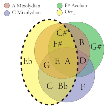
Example 1. Different scales combining to form a macroharmony

(click to enlarge)
[0.1] Macroharmony, as defined by Dmitri Tymoczko, is “the total collection of notes heard over moderate spans of musical time” (2011a, 4). Tymoczko makes a distinction between a macroharmony and a scale: whereas a scale is a type of musical ruler with increments or steps, macroharmony is more general, unrestricted by the number of objects within it or the distance between notes. As such, a scale can be part of a macroharmony, or a macroharmony can be part of a scale. For example, a polytonal piece simultaneously sounding two different scales forms a larger macroharmony (Example 1). Macroharmony is dynamic in that it constantly shifts as a piece progresses. Because of its flexibility, it is hard to classify movement between macroharmonic collections, let alone describe the macroharmony itself. Building primarily on the work of Ian Quinn (2006, 2007) and Jason Yust (2016), this paper demonstrates the utility of the discrete Fourier transform (DFT) for analyzing macroharmonies in a musically intuitive way while providing novel modes of hearing. I take a computational approach to assist in tracking the progression of macroharmonies. To begin, let’s examine a macroharmonic situation where traditional tools might prove insufficient.
Example 2. Requiem: Domine Jesu,

(click to enlarge)
[0.2] Example 2—mm. 31–34 of Domine Jesu from Maurice Duruflé’s Requiem, Op. 9 of 1947—shows a situation where the overarching macroharmony evades simple explanation by traditional tools.(1) The pitch content in the first two measures {A, B, D, E, G} is a subset of three A-centered diatonic scales: A dorian, mixolydian, and aeolian.(2) Measure 33 introduces
[0.3] In describing the effect octatonic and diatonic collections have on each other, Pieter van den Toorn (1983) uses the term interpenetration in the context of Stravinsky’s music. Using his approach, we might consider the passage in Example 2 as the overlapping union of two different scalar subsets: A mixolydian {A, B,
[0.4] The paper is formatted in three primary sections: Part 1 briefly introduces the DFT such that readers can interpret its calculations in terms of macroharmonic qualities; Part 2 discusses different methods for encoding the musical object—rather than representing PCs as there-or-not, one can allow for different PC weights; Part 3 shows that the DFT can serve as a systematic method for examining macroharmony through an analysis of Domine Jesu in Duruflé’s Requiem, Op. 9.
Part 1: Primer on the discrete Fourier transform
[1.0] Whereas most recording/sound engineers are familiar with the DFT’s use on audio waveforms, the analogous signal analyzed in music theory has been the PC set. A DFT on PCs returns 12 values, \(f_0-f_{11}\), corresponding to periodic intervals: \(f_n\) represents component n—a division of the PC-space into n parts. David Lewin (1959, 2001) was the first to propose the DFT for PC sets. Since this introduction to music theory, the DFT has been related to voice leading (Tymoczko 2008; Callender, Quinn, and Tymoczko 2008; Tymoczko and Yust 2019), and used for creating harmonic geometries and spaces (Yust 2015; Amiot 2016), defining and constructing balanced rhythms and scales (Milne et al. 2015), and describing stylistic trends and differences between composers (Yust 2019; Harding 2020). This project builds on Ian Quinn’s theory of chord quality (2007). Quinn shows that the DFT of a PC chord results in 6 non-trivial components (or values), \(f_1-f_6\), that each relate to qualitative genera.(5) Since each component corresponds to an even division of the space, calculating the DFT on chords approximating that division results in a high magnitude for that component.(6) For example, a major triad is a near-even division of the octave into three parts, and therefore it will have a high magnitude for \(f_3\).
[1.1] The current paper foregoes a detailed introduction to the mathematics of the DFT: For accessible external resources on understanding the DFT, I recommend Quinn (2006, 2007) for theoretical background and relationship to maximally even sets, Yust (2017b) for an analytic tutorial, and Callender (2007) to understand the mathematics. Additionally, Jenn Harding (2021) has created a user-friendly interactive web application for visualizing DFT components. This paper instead focuses on the interpretive and accessible takeaways by way of chord quality.
Example 3. DFT macroharmonic qualities

(click to enlarge)
[1.2] Chord qualities can be adapted to describe macroharmonies. Each component is associated with a macroharmonic quality: clustered quality, dyadicity, hexatonicity, octatonicity, diatonicity and whole-tone quality.(7) The first component (clustered quality) is notated \(f_1\), the second component (dyadicity) is notated \(f_2\), and so on. Example 3 shows each quality with its associated description. The DFT also returns \(f_0\), corresponding to a collection’s cardinality; we will discuss its particularities at the beginning of the analysis (Part 3).
[1.3] While there are prototypical scales that elicit high magnitudes for a particular component, macroharmonic collections vary in PC distributions and can result in high values for multiple components. For instance, in diatonic music, magnitudes for \(f_5\) and \(f_3\) both tend to be high. Does this suggest that the macroharmony evokes both diatonicity and hexatonicity, even though these two scales are often thought to be perceptually incongruous? I suggest two alternative interpretations for having high magnitudes for both \(f_5\) and \(f_3\). The first interpretation suggests that diatonicity isn’t just evoked solely with \(f_5\)—music emphasizing the circle of fifths—but through contribution of \(f_5\) and \(f_3\), challenging the preset, one-word qualities associated with each Fourier component. Under this interpretation, \(f_3\) might represents triadicity in a diatonic setting.(8) Hexatonicity would then be evoked only if \(f_3\) was high and \(f_5\) was low.(9) This interpretation describes qualities as emerging from the interaction between components and might be beneficial for classification tasks. An alternative, deconstructionist interpretation entertains a flexible listening of what diatonic and hexatonic collections usually mean—that is, we choose not to “flip the switch” between diatonic and hexatonic, but develop a fluid hearing for the intervallic makeup of each. I engage this issue directly in Part 3’s analysis of Duruflé’s Requiem, questioning these prototypical qualities and what they mean for us analytically as we begin to investigate results.
[1.4] Despite Amiot (2016) heralding the DFT as the “holy grail” of harmonic analysis, there have only been a handful of analyses. Out of the literature, the DFT has been applied analytically to the harmonic languages of Ligeti (Quinn 2007), Schubert (Yust 2015), Debussy (Yust 2017a), Crawford and Shostakovich, (Yust 2016), and, in a closing remark from Amiot (2017), Stravinsky. This paper adds to this growing discourse by providing a new computational methodology for analyzing music with the DFT.
Part 2: Data encoding and methodology
Example 4. Approaches to encoding music
(click to enlarge)
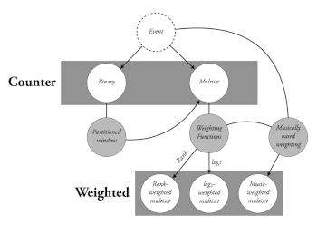
[2.0] Part 2 of this paper is divided into 3 sections, each covering a part of the encoding process for analysis: 1) binary vs. multiset approaches; 2) windowing; and 3) weighting. Example 4 shows a map of the encoding processes I discuss. An event, as shown at the top of Example 4, is a musical object comprised of different musical values such as pitch, duration, dynamic, or start-time. Although we can choose to study a variety of features from events, this paper focuses exclusively on PCs. Over the remainder of Part 2, I will discuss two types of PC array representations (shown as white nodes in Example 4): counter-type arrays, which count the frequency of events and weighted arrays, where events are encoded by certain rules or functions beyond their frequency. Weighting functions will be discussed later. The gray nodes show methods for weighting pitch information. All these methods for encoding and extracting PCs can predetermine the musical object, which directly affects DFT analysis.
2.1: Binary vs. multiset approaches
[2.1.0] In this paper, the input (or signal) we calculate the DFT on will always be a distribution of PCs. The characteristic function of a PC set is a 12-place vector \((p_0, p_1, \ldots, p_{11})\), where \(p_j\) is 1 if PC \(j\) is in the PC set and 0 otherwise.(10) For example, a C-major scale would be mapped as follows:
C major-scale:\(\{C, D, E, F, G, A, B\}\) \(\to\) characteristic function: \((1, 0, 1, 0, 1, 1, 0, 1, 0, 1, 0, 1)\)(11)
This representation is also known as a PC array.
[2.1.1] Representing the events as 1s and 0s is often called a binary or bit array in computer science. An encoding that allows values other than 1 and 0 is called a multiset array. A simple multiset—otherwise known as a frequency distribution—is a multiset which records the frequency of occurrences. Unless specified otherwise, when I use the term multiset I am referring to simple multisets. These counter-type binary and multiset arrays are used for various computational purposes, most notably in music for describing pitch-class profiles (Huron 2006; Temperley and Marvin 2008) and statistical learning models (Krumhansl 1990b; Saffran et al. 1999).
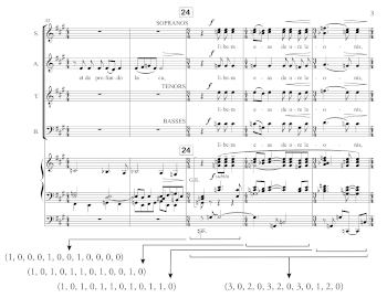
Example 5. Domine Jesu, rehearsal 24, binary vs. multiset
(click to enlarge)
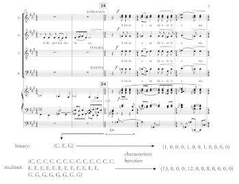
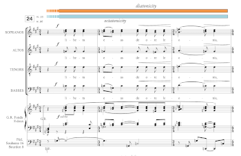
[2.1.2] Example 5 shows the difference between encoding rehearsal 24 of Duruflé’s Requiem with binary and multiset arrays. The music of rehearsal 24 marks a significant change: immediately prior, the organ has simple foundation stops—usually 8’ flutes and principals (no reeds)—on the Récit manual to accompany the altos’ solemn soli. Rehearsal 24 erupts with a dynamic change in texture and a shift to the Grand Choeur manual. To accompany the textural shift, the macroharmony moves from the previous collection, which contains A mixolydian with an added
[2.1.3] The impetus for multisetting is to move us away from conceiving macroharmonies as PC sets and towards viewing them ecologically—with variable distributions and emphases. Moving the musical object away from the ideal forms of macroharmony—that is, sets as binary collections—and towards observed musical objects marks a change in ideology; multisets permit more distinctions between sets to account for sensitivity to musical details.
2.2: Windowing
Example 6. Domine Jesu, melody at
(click to enlarge)
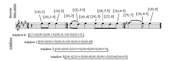
[2.2.0] Analytical findings are largely determined by segmentation procedures, and macroharmonic analysis is no exception. Though there is no standard procedure, the method should cater to the type of analysis and the music studied. Windowing is a procedure that segments the data into smaller, digestible pieces.(12) The method utilized here—overlapping sliding windows—imitates the experience of listening. Just as we take in pitch information and process it while listening to a piece, we can tell a computer to take a window spanning a certain number of beats and slide it through the score, one beat at a time, to retrieve pitch distributions. Example 6 shows how sliding windows extract pitch information from the melody at rehearsal 24 (from Example 5). First, the score is encoded as a discrete time-series (above the example) where each note onset has an associated time point written as [{PCs}, time point in quarter-note beats]. The windowing process (below the score) then groups adjacent time points into fixed-length segments. Example 6 shows the first 4 windows using a window length of 4 quarter notes.
Example 7. Domine Jesu, rehearsal 24, different window sizes

(click to enlarge)
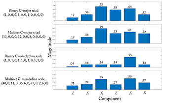
[2.2.1] The size of the window affects the results: shorter windows will show local harmonies while longer ones retrieve scales and/or macroharmonies. As Tymoczko (2011a) shows, changing window sizes shows different PC-distributions for different composers, conveying an element of musical style. Using multisets, Example 7 returns to rehearsal 24 to show the difference between a one-measure window and a three-measure window. This example simultaneously shows the usefulness of multisetting and windowing. The one-measure window retrieves a C-major triad, whereas a three-measure window shows a distribution resembling a C-mixolydian scale. For the three-measure window, a binary process retrieves (1, 0, 1, 0, 1, 1, 0, 1, 0, 1, 1, 0). This one characteristic function, however, can equally represent the other six modes with one flat (including both F major, C mixolydian, G dorian, etc.). By using a multisetting method, however, the tonic triad is emphasized through PC frequency: (40, 0, 11, 0, 36, 6, 0, 27, 0, 2, 6, 0). The method thus models how scale-degree frequency contributes to the sense of mode. To summarize the rationale thus far: larger windows highlight macroharmonic collections, while multisets emphasize the most frequently repeated notes.
Example 8. DFT calculations on different retrieval processes and window sizes for Domine Jesu, rehearsal 24
(click to enlarge)
[2.2.2] Window sizes therefore affect DFT calculations, and, by extension, our analytical interpretations. Example 8 shows a table of the DFT components pairing the two window sizes with the two counter arrays from Example 7. For ease of comparison, each component is normalized by the total cardinality, so that the maximum value for any magnitude is 1. The macroharmonic collection at rehearsal 24 evokes a diatonic atmosphere, so we should expect the DFT components to return high values for \(f_5\). Three of the four arrays result in a high magnitude for \(f_3\) and \(f_5\). Because the one-measure window only detects a triad—a near-even division of the octave into three parts—the values for \(f_3\) are prominent in the first two calculations. The three-measure binary window has a high \(f_5\) value, but \(f_3\) is not pronounced; the flat distribution encodes all PCs equally, and does not mark members of the tonic triad (or any triad for that matter) as any more significant. Since the three-measure multiset window captures both the diatonic distribution of PCs and pronounces the tonic triad through frequency, the DFT shows relatively high values for both \(f_3\) and \(f_5\). This demonstrates the efficacy of a larger window for capturing and describing macroharmony.
[2.2.3] Now we have a method to retrieve our data (windowing) and a way to encode it (multisetting). Since shorter windows observe verticalities and larger windows can be used for scales or collections, I implement a 12-beat window to capture the shifting umbra of macroharmony.(13) Unfortunately, while multisetting may seem effective at times, it is inconsistent and has glaring drawbacks. In Music and Probability, David Temperley warns that simple multisetting often misrepresents our experience of the music, particularly in key recognition: “the perception of key over a short segment of music. . . does not seem to be greatly affected by immediate repetitions or doublings of pitch-classes” (2007, 80). Frequency distributions count all PCs equally even when solely reinforcing a harmony—I call this the representation of repetition.(14) In short, the problem is that repetition does not necessarily equal cognitive salience or prominence. We see how multisetting goes awry in Example 7 (above). In the C-mixolydian multiset array, we might read the distribution as saying that scale degree is 20 times less prominent than scale degree , and scale degree is 6 times as prominent as scale degree .
[2.2.4] Are notes that are more common more prominent? It depends on what we mean by prominent. PCs that have a higher likelihood—represented with higher numbers in a frequency distribution—are more stable. In a sense, they are more important to maintain a collection. But once a harmonic setting is established, unexpected PCs are more jarring. This directs us to an important feature of information theory: the less probable an event is, the more surprising it is and the more information it yields (Meyer 1957). For our encoding method, this means less frequent events should be weighted more heavily. The next section discusses systems that account for pitch frequencies, but weight them by perceptual prevalence.
2.3: Weighting
[2.3.0] In data processing, weighting refers to a method of manipulating retrieved data. If we want to capture our experience of the ongoing macroharmony, the weighting procedure should shape the data according to our musical intuition. In this context, weighting acts as a filter that approximates the relative emphases a listener experiences.
[2.3.1] Until now, we have only used counter-type arrays (tallying frequencies). When events are weighted in terms other than their frequency of occurrence, I call the resulting array a weighted multiset: A weighted multiset shapes data according to predetermined rules or functions. There are countless possible weighting procedures. The two types of weightings this paper discusses are musically based and monotonic.
[2.3.2] Musical events have innumerable parameters that all interact to form the perception of sound. While counter methods are efficient when used appropriately, their simplicity can distort the data such that they don’t represent the experience of the sound.(15) In addressing such complications, some alternative methods weight events by predetermined knowledge-based rules (as per machine-learning engineers); I call these methods musically based weightings (shown in Example 4). Though I choose a different weighting approach in the analytical portion of the paper, musically based weightings are integral to the topic of data manipulation and I would be remiss not to discuss them here. Knowledge engineering—as it’s known in artificial intelligence research—normally designates the encoding of these specific rules to experts in the fields; similarly, these musically based weights should be predesigned by theorists or other music experts.(16) One example of a musically based weighting involves octave doubling: should pitches that are doubled at the octave count for two events? If not, instead of counting each separate event, a rule might collectively weight all instances of a pitch class as 1, regardless of how many octaves double it.(17)
Example 9. Weight by metric hierarchy
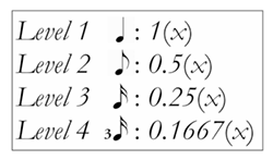
(click to enlarge)
[2.3.3] Knowledge-based systems (in the machine-learning sense of the word) in music assert the primacy of certain musical events and structures over others and correspondingly weight certain musical events more. We could easily design weighting procedures for different musical parameters such as duration, register, dynamic, syntax, etc. Say we wanted to design a system where meter influences a PC’s weight—the procedure could weight events higher when they coincide with stronger metric positions. One possible metric weighting would multiply the value of a note’s metric position by its share of the quarter note (Example 9). In other words, each PC is multiplied by a metric coefficient, weighting it a certain amount. A PC that lands on an eighth-note subdivision (such as the “and of 1”) would be weighted as .5. According to this procedure, the three-bar multiset from Example 7 would be weighted as (31, 0, 9, 0, 28.5, 6, 0, 18, 0, 2, 4.5, 0). This method of weighting is perceptually informed by listener attention, entrainment, and prediction research (London 2012), but, since these strong metric positions are likely to be members of the tonic triad (Prince and Schmuckler 2014), metric weighting may artificially overstate the tonic.(18) As Christopher Wm. White has shown (on music21’s Bach corpus), if we were to weight PCs metrically, the distribution would emphasize I, V and IV (respectively) of the home key (2018). This is a potentially valuable approach for research that concerns emphasized scale members, but because macroharmony’s object is a perceptual umbrella over time, our object ought to be flatter and more distributed. Deriving a musically based weighting system is complex: As perception is flexible, imprecise, and, ultimately, human, creating contextual “if . . . then” rules for each musical situation is an endless investigation. Accordingly, our model ought to prioritize a simple approach that controls for the representation of repetition and weights PCs by aural salience. For this reason, I implement a monotonic weighting procedure.
Example 10. Monotonic weightings of PC-frequency distributions, Domine Jesu, rehearsal 24

(click to enlarge)
[2.3.4] Applying monotonic functions to an array retains the order of numbers in relation to one another but alters their values. Example 10 shows a table of two monotonic functions—rank and \(log_2\)—that weight the counter-type multiset from rehearsal 24, beside the earlier stated metric-weighted multiset. Though working independently from the musical material, these monotonic functions are still musically intuitive, both retaining the relevance of frequent PCs and scaling for the representation of repetition. A rank-weighting system orders the values based on their respective frequencies. Ranking starts at the lowest-nonzero-frequency event and assigns it 1. It iterates the process to the next lowest frequency until all values are accounted for. As shown in Example 10, A is the least common note and is assigned 1,
Example 11. log2(x+1) function

(click to enlarge)
[2.3.5] Another effective monotonic function is the \(log_2(x+1)\) function—the weighting used in the following analysis.(20) I abbreviate \(log_2(x+1)\) as \(log_2\).(21) While one could easily use other commonly used logarithms (such as \(log_e\) or \(log_{10}\)), I choose \(log_2\) because its initial range for values is wider, allowing wider variance for lower values (Example 11). With \(log_2\) weighting, as the frequency for a single PC increases, its relative value for subsequent occurrences decreases. For instance, the value of a PC that occurs once is 1, but a PC that occurs five times is valued at 2.6. This makes musical sense: after establishing a macroharmony, repeating a pitch does little to perceptually disturb our sense of the macroharmony. With \(log_2\) weighting, the data reflects that infrequent PCs carry more information. In Example 7, the subtonic only occurs 6 times. Despite its low frequency,
Example 12. Domine Jesu, rehearsal 24, partitioned window
(click to enlarge)
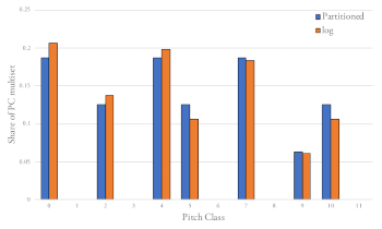
[2.3.6] \(log_2\) achieves similar results to an approach by David Temperley (2007). By building multisets from smaller binary windows, his method bypasses the weighting process by reorganizing the segmentation procedure—we might call this partitioned windowing. Example 12 demonstrates his approach. To examine the PC content in a three-bar window, we partition it into smaller binary windows; each smaller window adds together to form the cumulative multiset. In doing so, the resulting distribution is (3, 0, 2, 0, 3, 2, 0, 3, 0, 1, 2, 0). Temperley’s approach results in a multiset that has a .991 correlation to \(log_2\)’s array. This similarity is striking when normalized by the total cardinality, shown in Example 13. Both approaches serve as a failsafe to mitigate the distortional effects of counter methodology, but these operations occur at different stages of the retrieval process: partitioned windows extract counts, whereas \(log_2\) shapes an array post-extraction. As such, the methods are not mutually exclusive. A possible encoding procedure might include partitioned windows with both musically based and monotonic weighting. However, for the current analysis, \(log_2\) weighting is simple, efficient, and clear for describing macroharmony.
Example 13. Domine Jesu, rehearsal 24, partitioned window vs. log2
(click to enlarge) | Example 14. Coding procedure flow chart
(click to enlarge) |
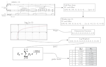
[2.3.7] We can now implement the methodology for analysis. Example 14 shows a flow chart summarizing the coding process.(22) The process is as follows: (1) extract all PCs and their respective positions (offsets) from the score (as a discrete time series); (2) divide the data into windows of 12 beats; (3) append PC frequency to a PC array; (4) weight the arrays (\(log_2\)); and (5) calculate the DFT on each window.(23)
Part 3: Analysis of Domine Jesu
[3.0.0] In analyzing the Domine Jesu with the methodology just presented, I will demonstrate that the DFT can be used to illuminate elements of Duruflé’s macroharmonic language, suggesting its broader applicability. After providing context (3.1)—including background on Duruflé, research on the Requiem, a formal analysis of the piece, and results of the analytical methodology—the analysis consists of 4 sections. The first three sections show that the DFT identifies macroharmonies operating at a functional and formal-functional level (3.2), macroharmonic foreshadowing (3.3), and ambiguity caused by macroharmonic pivots (3.4). The final section (3.5) synthesizes these techniques and observations.
3.1 Contexts and components
[3.1.0] Maurice Duruflé was a 20th century organist who studied with Charles Tournemire, assisted Louis Vierne at Notre Dame, and is often grouped with the French organ school (including Vierne, Charles-Marie Widor, and Marcel Dupré). Though his oeuvre is small, Duruflé’s style is distinct from that of the other French organists: it is less improvisatory and juxtaposes modal themes with 20th century techniques—showcased in the Requiem, Op. 9, Quatre Motets, Op. 10, and Cum Jubilo, Op. 11.(24) He is celebrated for his organ works and his frequently performed Requiem.(25) The Requiem is a harmonization of the Gregorian chant “Missa pro defunctis” from the Liber Usualis. Duruflé uses church modes as well as hexatonic, octatonic, and whole-tone collections to harmonize the chant. Domine Jesu includes both subtle and precipitous transitions between macroharmonic collections, making it a great choice for macroharmonic analysis with the DFT.
[3.1.1] Despite the Requiem’s success, it has received little analytical attention. Most publications on the piece concern biographical information (Ebrecht 2002) or interpretive cues for performers and conductors (Cooksey 2000, Kano 2004). James Frazier (2007), for example, provides a comprehensive background of Duruflé and the history of the Requiem. Though the book doesn’t focus on analysis, he alludes to the importance of macroharmony in the piece: “The genius of the Requiem lies in the modal ‘harmony’ merely implied in the purely horizontal, medieval melodies. . . ” (168). The most notable analytic writing on the Requiem is by Daniel Harrison in Pieces of Tradition (2016). As part of a larger project on extended tonality, Harrison studies tonal hierarchies “congruent with the overtone-series hierarchy,” or what he calls “overtonality,” in 20th century music (2016, 17). Harrison looks at two movements from the Requiem—the “Introit” and “In paradisum.” Both movements are generally more vertically harmonic than Domine Jesu, so the choice is logical considering his analytical apparatus prioritizes verticalities and tonal alterations. For example, in his analysis of the “Introit’s” opening, he reduces the harmonic structure to basic triads with extensions. His goal is essentially interpretive, suggesting that changes to the harmonic structure change the color of the chord. Harrison’s approach and mine both use prototypical objects to describe the qualitative experience of larger collections. However, Harrison relates pitches to the overtone series, whereas DFT macroharmonic quality relates pitches to symmetrical collections.
Example 15. Domine Jesu, form chart

(click to enlarge)
Example 16. Domine Jesu, magnitude values

(click to enlarge)
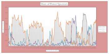
Example 17. Domine Jesu, share of power for f0–f6 (separated)

(click to enlarge)
Example 18. Domine Jesu, share of power for f3, f4, and f5 (compounded)
(click to enlarge)
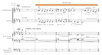
[3.1.2] Since the sung melody of the Requiem is taken from a Gregorian chant that lacks a clear form, the form is defined by Duruflé’s additions; the upper portion of Example 15 shows the form as shaped by Duruflé’s additional melodic content, texture, and harmonization. The global form is A-B, where A is partitioned further into a-b-a’ and B divides into c-d-e-d. The A section (mm. 1–97) is largely either diatonic or octatonic, with jarring shifts and moments of high energy. The B section (mm. 98–169) contains hexatonic, diatonic, and octatonic collections, but is often ambiguous. Its thinned, drawn out texture, and nasal reed stops (crumhorn and vox humana) accompany a baritone soloist, who embodies prophesying with a droning melody. The subsequent analysis contextualizes the macroharmony—shown in the lower portion of Example 15—with the form of the piece, demonstrating how it works to reinforce elements of the form. Let us begin with the DFT results from our coding procedure.
[3.1.3] The code, as described in Part 2, yields magnitude values for each window. Examples 16, 17 and 18 show the data graphically. The y-axes differ between charts, but the x-axes always represent time, organized by each window’s starting beat. To represent windows in the graphs, I use the notation: “w.(starting position in beats).” Example 16 shows the initial results of the calculation, which are somewhat hard to read. Because \(f_0\) is the cardinality, it always has the highest magnitude and eclipses the other components. Instead, it’s easier to separate the components into their own graphs, and square their respective magnitude values. Clifton Callender points out that this pronounces the most active components, making them “pop out” (2007). Squaring the magnitudes of the DFT yields the power spectrum.(26) In Example 17, each component is normalized to represent a percentage of the power spectrum (y-axis). A particular component peaking in the graph means that it occupies more of the power spectrum, ostensibly accompanied by the corresponding quality. Because of the normalization procedure, there are a few differences between Example 16 and 17: for example, in w. 271 of Example 16, \(f_5\) maintains a relatively level magnitude for the following 10 windows, but in the same windows in Example 17, \(f_5\) leaps upward. This disparity means that even though the magnitude remains the same, \(f_5\) briefly occupies more of the power spectrum (due to the lower cardinality in the window). Normalizing by total power shifts \(f_0\) from representing cardinality to something akin to chromaticity (or chromatic saturation): more evenly spread PC distributions have greater shares of their power in \(f_0\).(27) Therefore, \(f_0\) is represented in Example 17 as well. The y-axes in Example 17 are scaled for visual accessibility, but this also means it’s more difficult to see which components hold a larger share of power; a relatively high peak in one component can still be lower than a relatively low peak for another component. This article primarily focuses on the three components that bring out the piece’s macroharmonic contrast the most—f3 (hexatonicity), \(f_4\) (octatonicity), and \(f_5\) (diatonicity)—with occasional supplemental discussion of other components. Example 18 plots these three components together, and is the primary basis of the analysis. The remaining musical examples incorporate color-coded windows corresponding to Examples 16–18.
3.2 Macroharmonic antitonics and formal function
[3.2.0] In examining Example 18, we notice that octatonicity (\(f_4\)) always leads to diatonicity; any peak in blue is followed by orange. This shows a unidirectional, even functional relationship between the two collections—that is, octatonic macroharmonies move to diatonic ones, but not necessarily the other way around. Harrison has made the argument that in the 20th century, harmonic function can be “reinscribed as collectional (and even macroharmonic) contrast” (2016, 132). Using Harrison’s terminology, in Domine Jesu the diatonic collection functions as a stable tonic whereas the octatonic collection functions as an antitonic.
[3.2.1] Comparing Example 18 to Example 15 reveals that this macroharmonic-functional relationship is also related to the work’s form: Not only do the octatonic collections precede diatonic ones, but they also herald sectional divisions. Any use of the octatonic cues the end of one section and signals the next (diatonic) one—this is clear from the gray comments in Example 16. The octatonic’s antitonic function is therefore analogous to how—in the tonal tradition—a dominant often marks the end of one section, and the tonic initiates the subsequent unit.
Example 19. Domine Jesu, mm. 1–16

(click to enlarge)
[3.2.2] The introduction of the piece (Example 19) clearly evokes Oct01 with its subset {A,
3.3 Rehearing, subliminality, and manifestation
[3.3.0] In the moment, the Ds in m. 8 sound like chromatic passing tones between
[3.3.1] The collection in w. 21 (mm. 7–12) has 5 PCs: {
[3.3.2] Using the example at hand in mm. 7–12: even though E doesn’t fit into the hexatonic, the other notes do, making the collection a near match. Because the DFT’s components are continuous divisions of the space, inclusion relationships do not fully determine proximity between sets; using the DFT fuzzies the boundary and invites interpretation rather than saying whether a set is or is not contained within another (such as the introduction’s example).(29) Hearing the subliminal shadow of Hex12 in the beginning primes us for the appearance of the hexatonic scale later in the piece.
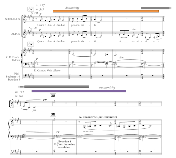
Example 20. Domine Jesu, mm. 117–131
(click to enlarge and see the rest)
[3.3.3] The explicit manifestation of the hexatonic (Hex03) surfaces in the e section shown in Example 20.(30) The e section contains the most macroharmonic shifts in the piece, moving between hexatonic, octatonic, and diatonic. Just prior to the minor third at rehearsal 38, the music is in E ionian (section d). To transition, toggles between
3.4 Macroharmonic pivots and ambiguity
[3.4.0] The pivoting third (in Example 20), which eventually leads into the hexatonic section, prepares the macroharmonic change by encouraging ambiguity: coming from a diatonic setting, it initially sounds as a drone from E minor, but as the crumhorn imposes hexatonicity, we recognize the minor third as a pivot between diatonic and hexatonic macroharmonies. This ambiguity is also shown by the DFT. The ambiguity of the stagnant, pivoting minor third shown in the gray window (Example 20) appears in Example 18 as a relatively high point for diatonicity, octatonicity, and hexatonicity. The relatively high levels for \(f_3\)–\(f_5\) might be better contextualized with \(f_0\) (Example 17). Because the power is distributed into fewer PCs, the share of power that each component possesses is raised. So, the ambiguous representation of the minor third is represented as the combination of a low magnitude for \(f_0\) and high values for \(f_3-f_5\).
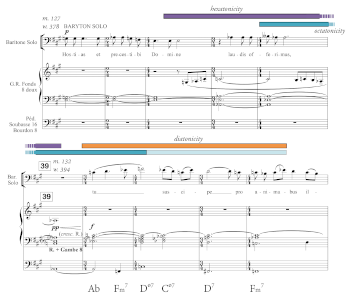
Example 21. Domine Jesu, mm. 127–136
(click to enlarge)
[3.4.1] The baritone soloist enters the hexatonic texture in measure 127—five measures after the crumhorn’s initial entry (Example 21). As the texture expands, the local harmonies quickly shift, affecting the macroharmony. Bridging the established hexatonic with the subsequent diatonic in measure 133, the window (w. 390) starting in m. 131 identifies high octatonicity. Since the window spans two scalar collections, it adds pitches from both: mixing the hexatonic from the crumhorn and soloist with the subsequent
3.5 “From death to life”: Conceptual assembly
Example 22. Domine Jesu, mm. 35–41
(click to enlarge and see the rest)
[3.5.0] Just as Hex03 manifests after a subliminal relation, a similar foreshadowing-realization situation occurs between the examples which started our inquiry: m. 31 (Example 2) and m. 35/reh. 24 (Examples 5, 7 and 10). In m. 31 (w. 83), the graph shows high diatonicity (\(f_5\)) with subliminal octatonicism (\(f_4\)). Immediately afterward, the music shifts away from A mixolydian, bursting into C mixolydian at reh. 24 (recreated in Example 22)—the musical excerpt used earlier to demonstrate windowing and weighting. The jarring shift, reinforced by the subito forte, only contains a few common tones between the scales (including the E4 in the melody).(32) However, C mixolydian retains the same subliminal octatonicism as A mixolydian. Only a few measures later, Oct01 emerges in measure 38–41, and \(f_4\) spikes accordingly.(33)
Example 23. Macroharmonic subset relationships
(click to enlarge)
[3.5.1] Oct01’s surfacing (at rehearsal 25) links the A mixolydian at rehearsal 24 to the sudden C mixolydian shift through common tones. Despite the A and C mixolydian scales only sharing 4 common tones {D, E, G, A}, the subliminal Oct01 that connects them contains 5 PCs from each (Example 23)—a result of its transpositional symmetry (T3). In fact, it contains mode-defining scale degrees of each key, including ,, to define the tonic triad and ,—where the seventh scale degree denotes the mixolydian mode. In Domine Jesu, the octatonic works as a subliminal backdrop to the entire a section. Originally set up with the introduction, the macroharmonic sinew lies beneath the surface through
Example 24. Domine Jesu, mm. 145–158
(click to enlarge and see the rest)
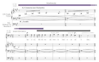
[3.5.2] Prior to the final d section, Hex03 and Oct12 appear consecutively (Example 24). Hex03 returns first, accompanied by the distinct crumhorn stop and E3/G3 minor third that appeared with its initial entry. The baritone soloist enters in measure 148, still retaining Hex03 with the exception of a passing
Example 25. Domine Jesu, mm. 159–169
(click to enlarge and see the rest)
[3.5.3] To conclude the movement, the Oct12 in e fulfills its macroharmonic antitonic function, leading to the final diatonic section in
4. Conclusion
[4.0] While this paper presents a novel methodology for studying macroharmony, its rigor also restricts its analytical expressiveness. There are two places in the methodology to explore further. First, preset methods for weighting multisets and segmenting the music via window size approximate the perceptual experience of macroharmony, but human perception is not a fixed input system. For example, experiencing the same thing multiple times changes our understanding of it: expectation “sometimes behaves so strangely” (Deutsch 1995). The retrieval and/or analytical methodology might be further adapted to reflect that experience. One possible change might be in the windowing procedure. Using variable window sizes might represent our perception more accurately than a fixed window. Perhaps reinforcement of a particular frequency distribution—pitches sounding within the active collection—allows our cognitive window to project further, while introduction of new pitches reorients our attention to more local macroharmonies. Sudden changes in texture, tempo, dynamics, or contour might also affect our cognitive window.(34)
[4.1] Second, as mentioned earlier, the \(log_2\) method may be supported by information theory, but the model here focuses only on PCs, an idealistic musical object. This eliminates the effect of any stylistic musical elements, such as timbre, register, acoustics, etc. Our perception is also changed by context and the interaction between musical parameters. For example, the same melody can be interpreted completely differently in a different metric context. An ideal weighting system should be flexible enough to accommodate these different contexts.
[4.2] But perhaps the discrepancy between our experience and the present encoding method is an opportunity to direct our analytical gaze; confronting whether the results are musically insightful or intuitive can teach us about the music and our cognition. In modeling music computationally, I’ve found that the most interesting results happen when the calculations actually misalign with my musical intuition.
[4.3] One moment of stark contrast between my hearing of Domine Jesu and the graphs is at rehearsal 24—the example used for windowing and weighting (and Example 23). The sudden transition to rehearsal 24 presents two distinct textures and dynamics. Counterintuitively, because the windows blend A and C mixolydian for a moment, Example 19 (ww. 89–99) shows a decrease in diatonicity, even though I feel overwhelmed by diatonicism. The encoding procedure overlooks the extreme contrast in texture, and the windowing procedure mixes two distinct sections. Then, the graph shows a substantial change moving into the following octatonicity—a moment which sounds smooth due to the descending melodic contour and textural continuity. Rather than using these moments of discontinuity to discredit the methodology or refute our intuition, we should use them to question our values as analysts and listeners, grappling with how distances between models and our personal experience shape our individual musical identities.
Matt Chiu
Department of Music Theory
Eastman School of Music
University of Rochester
40 Falstaff Rd., Rochester, NY 14609
mchiu9@u.rochester.edu
Works Cited
Amiot, Emmanuel. 2016. Music Through Fourier Space: Discrete Fourier Transform in Music Theory. Springer. https://doi.org/10.1007/978-3-319-45581-5.
—————. 2017. “Interval Content vs. DFT.” In Mathematics and Computation in Music, ed. Octavio A. Agustín-Aquino, Emilio Lluis-Puebla, and Mariana Montiel, 151–66. Springer. https://doi.org/10.1007/978-3-319-71827-9_12.
Callender, Clifton. 2007. “Continuous Harmonic Spaces.” Journal of Music Theory 51 (2): 277–332. https://doi.org/10.1215/00222909-2009-004.
Callender, Clifton, Ian Quinn, and Dmitri Tymoczko. 2008. “Generalized Voice-Leading Spaces.” Science 320 (5874): 346–48. https://doi.org/10.1126/science.1153021.
Clough, John, and Jack Douthett. 1991. “Maximally Even Sets.” Journal of Music Theory 35 (1/2): 93–173. https://doi.org/10.2307/843811.
Conklin, Darrell, and Ian Witten. 1995. “Multiple Viewpoints Systems for Music Prediction.” Journal of New Music Research 24 (1): 51–73. https://doi.org/10.1080/09298219508570672.
Cooksey, Karen Lou. 2000. “The Duruflé Requiem: A Guide for Interpretation.” Undergraduate Honors Thesis Collection at Butler University.
Cuthbert, Michael Scott and Christopher Ariza. 2010. “music21: A Toolkit for Computer-Aided Musicology and Symbolic Music Data.” In Proceedings of the 11th International Society for Music Information Retrieval Conference: 637–642.
Deutsch, Diana. 1995. Musical Illusions and Paradoxes. Philomel Records.
Ebrecht, Ronald. 2002. Maurice Duruflé, 1902–1986: The Last Impressionist. Scarecrow Press.
Forte, Allen. 1973. The Structure of Atonal Music. Yale University Press.
Frazier, James E. 2007. Maurice Duruflé: The Man and His Music. University of Rochester Press.
Harding, Jenn. 2020. “Computer-Aided Analysis Across the Tonal Divide: Cross-Stylistic Applications of the Discrete Fourier Transform.” Conference Proceedings of the Music Encoding Conference at Tufts University. http://dx.doi.org/10.17613/2n0b-1v04.
—————. 2021. “Jenn’s Visual Pitch Class Vector Calculator.” http://www.jenndharding.com/vectorcalculator.
Harrison, Daniel. 2016. Pieces of Tradition: An Analysis of Contemporary Tonal Music. Oxford University Press. https://doi.org/10.1093/acprof:oso/9780190244460.001.0001.
Huron, David. 2006. Sweet Anticipation: Music and the Psychology of Expectation. MIT Press. https://doi.org/10.7551/mitpress/6575.001.0001.
Kano, Thea. 2004. “Visions of a Tranquil End: The Expressive and Stylistic Interpretation of Maurice Duruflé’s Requiem, Opus 9.” DMA diss., University of California, Los Angeles.
Krumhansl, Carol L. 1990a. Cognitive Foundations of Musical Pitch. Oxford University Press. https://doi.org/10.1093/acprof:oso/9780195148367.001.0001.
—————. 1990b. “Tonal Hierarchies and Rare Intervals in Music Cognition.” Music Perception 7 (3): 309–24. https://doi.org/10.2307/40285467.
Lerdahl, Fred, and Ray Jackendoff. 1983. A Generative Theory of Tonal Music. MIT Press. https://doi.org/10.7551/mitpress/12513.001.0001.
Lewin, David. 1959. “Re: Intervallic Relations between Two Collections of Notes.” Journal of Music Theory 3 (2): 298–301. https://doi.org/10.2307/842856.
—————. 2001. “Special Cases of the Interval Function between Pitch-Class Sets X and Y.” Journal of Music Theory 45 (1): 1–29. https://doi.org/10.2307/3090647.
London, Justin. 2012. Hearing in Time: Psychological Aspects of Musical Meter. Oxford University Press. https://doi.org/10.1093/acprof:oso/9780199744374.001.0001.
Meyer, Leonard B. 1957. “Meaning in Music and Information Theory.” The Journal of Aesthetics and Art Criticism 15 (4): 412–24. https://doi.org/10.1111/1540_6245.jaac15.4.0412.
Milne, Andrew J., David Bulger, Steffen A. Herff, and William A. Sethares. 2015. “Perfect Balance: A Novel Principle for the Construction of Musical Scales and Meters.” In Mathematics and Computation in Music, ed. Tom Collins, David Meredith, and Anja Volk, 11 (1–2): 101–33. Springer. https://doi.org/10.1007/978-3-319-20603-5_9.
Morris, Robert D. 1987. Composition with Pitch Classes: A Theory of Compositional Design. Yale University Press. https://doi.org/10.2307/j.ctt1xp3ss4.
Prince, Jon B., and Mark A. Schmuckler. 2014. “The Tonal-Metric Hierarchy: A Corpus Analysis.” Music Perception 31 (3): 254–70. https://doi.org/10.1525/mp.2014.31.3.254.
Saffran, Jenny R., Elizabeth K. Johnson, Richard N. Aslin, and Elissa L. Newport. 1999. “Statistical Learning of Tone Sequences by Human Infants and Adults.” Cognition 70 (1): 27–52. https://doi.org/10.1016/s0010-0277(98)00075-4.
Straus, Joseph N. 1984. “Review of The Music of Igor Stravinsky by Pieter C. van den Toorn.” Journal of Music Theory 28 (1): 129–34. https://doi.org/10.2307/843455.
Studer, Rudi, Richard V. Benjamins, and Dieter Fensel. 1998. “Knowledge Engineering: Principles and Methods.” Data and Knowledge Engineering 25 (1–2): 161–97. https://doi.org/10.1016/s0169-023x(97)00056-6.
Temperley, David. 2007. Music and Probability. MIT Press. https://doi.org/10.7551/mitpress/4807.001.0001.
Temperley, David, and Elizabeth West Marvin. 2008. “Pitch-Class Distribution and the Identification of Key.” Music Perception 25 (3): 193–212. https://doi.org/10.1525/mp.2008.25.3.193.
Tymoczko, Dmitri. 2008. “Set-Class Similarity, Voice Leading, and the Fourier Transform.” Journal of Music Theory 52 (2): 251–72. https://doi.org/10.1215/00222909-2009-017.
—————. 2011a. A Geometry of Music: Harmony and Counterpoint in the Extended Common Practice. Oxford University Press.
—————. 2011b. “Round Three.” Music Theory Spectrum 33 (2): 211–15. https://doi.org/10.1525/mts.2011.33.2.211.
Tymoczko, Dmitri, and Jason Yust. 2019. “Fourier Phase and Pitch-Class Sum.” In Mathematics and Computation in Music, ed. Mariana Monteil, Francisco Gomez-Martin, and Octavio Agustín-Aquino. Lecture Notes in Computer Science, 11502: 46–58. Cham. https://doi.org/10.1007/978-3-030-21392-3_4.
Quinn, Ian. 2006. “General Equal-Tempered Harmony: Introduction and Part I.” Perspectives of New Music 44 (2): 114–58.
—————. 2007. “General Equal-Tempered Harmony: Parts 2 and 3.” Perspectives of New Music 45 (1): 4–63.
Van den Toorn, Pieter C. 1983. The Music of Igor Stravinsky. Yale University Press.
White, Christopher Wm. 2018. “Meter’s Influence on Theoretical and Corpus-Derived Harmonic Grammars.” Indiana Theory Review 35 (1–2): 93–116. https://doi.org/10.2979/inditheorevi.35.1-2.04.
Yust, Jason. 2015. “Schubert’s Harmonic Language and Fourier Phase Space.” Journal of Music Theory 59 (1): 121–81. https://doi.org/10.1215/00222909-2863409.
—————. 2016. “Special Collections: Renewing Set Theory.” Journal of Music Theory 60 (2): 213–62. https://doi.org/10.1215/00222909-3651886.
—————. 2017a. “Harmonic Qualities in Debussy’s ‘Les sons et les parfums tournent dans l’air du soir.’” Journal of Mathematics and Music 11 (2–3): 155–73. https://doi.org/10.1080/17459737.2018.1450457.
—————. 2017b. “Review of Emmanuel Amiot, Music Through Fourier Space: Discrete Fourier Transform in Music Theory (Springer, 2016).” Music Theory Online 23 (3). https://doi.org/10.30535/mto.23.3.12.
—————. 2019. “Stylistic Information in Pitch-Class Distributions.” Journal of New Music Research 48 (3): 217–31. https://doi.org/10.1080/09298215.2019.1606833.
Footnotes
* A portion of this paper was presented at Music Theory Midwest, University of Cincinnati (May 10–11, 2019). I would like to thank Zachary Bernstein and Eron F.S. for their editorial comments on various editions of this paper, Jason Yust for introducing me to the DFT, and the members of First Parish Church in Weston, MA who gave me the chance to perform Duruflé’s Requiem in 2018.
Return to text
1. The “w.” in the figure stands for “window” and will be made clear later.
Return to text
2. The collection also fits neatly in a G pentatonic with A as its center—otherwise known as A dorian pentatonic—but because the macroharmony expands, I find a subset interpretation more applicable.
Return to text
3. This same issue is addressed in Tymoczko 2011b.
Return to text
4. These issues are particularly relevant to other 20th century composers. For example, many readers will draw connections to Messiaen, whose “charm of impossibilities” relies on the play between diatonic and symmetrical scales.
Return to text
5. Quinn (2007) relates DFT components to qualities by building on Clough and Douthett (1991), making a one-to-one correspondence with maximally even subgenera.
Return to text
6. Quinn initially discusses each component in terms of balance (as Fourier properties). When interested in only the quality, as we are here, “we begin with the two-dimensional quality of the tipping force (direction and magnitude) and reduce it to one dimension by throwing out the direction component” (59). The directional component is known as phase, and is beyond the scope of this paper.
Return to text
7. Different sources use different quality labels for components. \(f_1\) is often labeled as chromaticity, but macroharmonic collections are different than the vertical slices often analyzed. As a high magnitude for \(f_1\) requires chromatically adjacent PCs, it captures a clustered quality for macroharmony.
Return to text
8. I borrow the term triadicity from Yust (2017a, 2019). Yust discusses \(f_3\) in diatonic music, stressing major and minor thirds. Carol Krumhansl (1990a) noted that a Fourier transform of key-profiles (derived by probe-tone studies) would find two strong components—\(f_5\) and \(f_3\). In the context of key-profiles, \(f_3\) represents a circle of thirds.
Return to text
9. Amiot (2017) describes \(f_3\) in its non-tonal context with augmented triads or the hexatonic scales (Napoleon hexachord).
Return to text
10. In this formulation, incidentally, the characteristic function is technically a vector rather than a function. The term has sometimes been used this way in the DFT literature, but strictly speaking, mathematicians might prefer to call it a characteristic vector.
Return to text
11. This is also known as a characteristic map of the C-major scale onto \(\mathbb{Z}_{12}\).
Return to text
12. In this context, the term window refers to partitioning the data stream; it is unrelated to the parallel apodization/tapering function in signal processing.
Return to text
13. Obviously, window type and window size affect the PC distributions. Exploration of these windowing procedures and the differences between yielded results would be a fruitful study (see chapter 5 of Tymoczko 2011a for a cursory discussion on the topic). In the analysis portion of this paper, there was, however, little difference between windows whose size was within 4; the analysis portion of the paper uses a window size of 12 beats to analyze Domine Jesu—neither windows of length 8 or 16 changed the results significantly. One reason for the consistent results, despite the window size, is the \(\log_2\) weighting procedure (discussed subsequently).
Return to text
14. One possible solution to the representation of repetition is by weighting each PC by its duration rather than its frequency of occurrence. This procedure may run into its own issues; for example, does a pedal tone influence the ongoing collection more than the notes being introduced above it?
Return to text
15. Conklin and Witten (1995) use counter methodology, contextual probability (n-grams), and the interaction of musical parameters to form their multiple viewpoint systems.
Return to text
16. For more detail about knowledge-based engineering, see Studer, Benjamins, and Fensel (1998). Knowledge-based rules are methods of shaping objects so as to replicate our experience of them. The validity of a knowledge system is evaluated on its correlatation to our subjective experience.
Return to text
17. Certain “Preference Rules” from Lerdahl and Jackendoff’s A Generative Theory of Tonal Music (1983) can be re-coded as knowledge-based rules if designed more rigorously.
Return to text
18. The corpus used for Prince and Schmuckler consisted of piano works from Bach to Scriabin. As compositional probabilities change between styles, musically based weightings—including the proposed metric weighting—should be adjusted per the repertoire.
Return to text
19. In music theory, contour theory is a system analogous to rank weighting (Morris 1987).
Return to text
20. Though log-weighting is common in various other fields, I have not yet encountered its use in music analysis.
Return to text
21. 1 must be added before calculating \(\log_2(x)\) because \(\log_2(0)\) is undefined—meaning the function wouldn’t work if there was a single PC missing from any window.
Return to text
22. In Example 14, \((f_0, f_1, \ldots , f_6)\) is the DFT of a characteristic function \((p_0, p_1, \ldots, p_{12})\). The formulation to the left of Example 14 yields a complex number. It is more useful here to represent values in polar form—containing, as shown on the right, magnitude \(|f_n|\) and phase \(n\). As previously mentioned, for this paper’s purposes we ignore the phase element.
Return to text
23. The initial pitch extraction uses music21—a python toolkit developed at MIT (Cuthbert and Ariza 2010).
Return to text
24. Duruflé has 14 opus numbers as well as a few compositions published posthumously.
Return to text
25. There are three orchestrations of the Requiem: (1) for full orchestra and organ, (2) for reduced orchestra and organ, and (3) for solo organ. The analysis in the paper uses the solo organ score.
Return to text
26. The power spectrum is the sum of squared magnitudes. The Parseval-Plancherel identity says that the DFT preserves power (the sum of squared magnitudes = the sum of squared PC weights).
Return to text
27. This also means that chromatic distributions of PCs will have lower magnitudes overall (except \(f_0\)).
Return to text
28. Given the modal style of composition, I default to mode names for labeling.
Return to text
29. Yust (2016) shows the DFT can even calculate proximity of collections without any common tones.
Return to text
30. The manifestation is a different hexatonic scale than the earlier subliminal relation—Hex03 instead of the earlier Hex12—foreshadowing the abstract concept of a hexatonic, not the specific Hex03. However, there is another comparative connection between the hexatonics and their common-tone contexts. Every diatonic collection shares four pitch classes with two different hexatonic collections. Hex03 has four common tones with the adjacent diatonic collection E major just as Hex12 has four common tones with its adjacent diatonic F# natural minor.
Return to text
31. The chords are annotated by collection—meaning the bass is ignored—in a pseudo-jazz-chord formatting: 7 implies a minor seventh.
Return to text
32. Even though the shift is jarring, the magnitude for \(f_5\) remains high because the collection is still diatonic. If weighted equally, the magnitude for all diatonic collections is equal.
Return to text
33. Though m. 38 is not entirely octatonic, the following three octatonic measures overwhelm the window’s macroharmony with Oct01.
Return to text
34. Another windowing approach might adjust with tempo fluctuations to reflect the bandwidth of perceptual entrainment. Adjustable window sizes are called session windows.
Return to text
Copyright Statement
Copyright © 2021 by the Society for Music Theory. All rights reserved.
[1] Copyrights for individual items published in Music Theory Online (MTO) are held by their authors. Items appearing in MTO may be saved and stored in electronic or paper form, and may be shared among individuals for purposes of scholarly research or discussion, but may not be republished in any form, electronic or print, without prior, written permission from the author(s), and advance notification of the editors of MTO.
[2] Any redistributed form of items published in MTO must include the following information in a form appropriate to the medium in which the items are to appear:
This item appeared in Music Theory Online in Volume 27, Issue 3 in September 2021. It was authored by Matt Chiu (mchiu9@u.rochester.edu), with whose written permission it is reprinted here.
[3] Libraries may archive issues of MTO in electronic or paper form for public access so long as each issue is stored in its entirety, and no access fee is charged. Exceptions to these requirements must be approved in writing by the editors of MTO, who will act in accordance with the decisions of the Society for Music Theory.
This document and all portions thereof are protected by U.S. and international copyright laws. Material contained herein may be copied and/or distributed for research purposes only.

Prepared by Michael McClimon, Senior Editorial Assistant
Number of visits:
12667