Chord Proximity, Parsimony, and Analysis with Filtered Point-Symmetry
Richard Plotkin
KEYWORDS: maximal evenness, voice-leading parsimony, neo-Riemannian theory, transformational theory
ABSTRACT: Filtered Point-Symmetry (FiPS) is a tool for modeling relationships between iterated maximally even sets. Common musical relationships can be studied by using FiPS to model chords contained within a specific scalar context (such as C major or the 01-octatonic collection), and by capturing those relationships in a FiPS configuration space. In this work, many FiPS configuration spaces are presented; some are isomorphic to commonly referenced voice-leading spaces like the neo-Riemannian Tonnetz, and others show tonal networks that have not previously been explored. A displacement operation is introduced to codify the traversal of a configuration space, and a short music analysis is provided to demonstrate some benefits of the approach.
DOI: 10.30535/mto.25.2.3
Copyright © 2019 Society for Music Theory
[1.1] Scale theory and transformational theory have converged in some interesting and exciting ways in music theory, notably in the presentation of neo-Riemannian theory and other transformational theories involving frugal pitch-class changes (where “frugal” here is meant to include, but not exclusively refer to, parsimonious voice leading). An important visualization of this convergence is the neo-Riemannian Tonnetz, which ushered in a wave of thought about how music moves in time through a constructed (or generated) space. In many of these constructions, there is a substantive reliance on the relative evenness of a collection of pitches or pitch classes. I want to draw your attention to three particular approaches, the last of which will be the focus of this article.
[1.2] First, Jason Yust’s approach to discrete Fourier transform (DFT) phase space (Yust 2015b): the DFT, as discussed by David Lewin (2001) and, later, Ian Quinn (2006, 2007), can give us a relative numeric representation of evenness in any pc set. Broadly, it allows us to parse evenness along a clear continuum relative to a totally even distribution. Additionally, while two different whole tone collections would have the same magnitude of evenness as measured by the DFT, the phases of those collections would be in opposition. Yust, in DFT phase space, explores how phases from the DFT tell a story about harmonic relationships. Second, the Callender, Quinn, and Tymoczko (CQT) (2008) approach to voice-leading space: As with DFT phase space, the voice-leading space constructed by Callender, Quinn, and Tymoczko maintains evenness as a core principal, and distances between elements involve considerations of near-evenness and note-to-note proximity. Lastly, the approach to modeling iterated maximally even sets through Filtered Point-Symmetry: Filtered Point-Symmetry, or “FiPS,” is a transformational system built upon the manipulation of iterated maximally even sets over time. It is a geometric visualization of John Clough and Jack Douthett’s (1991) $J$ function.
[1.3] This article deeply examines the utility of FiPS-based models. Although some models overlap with those that can be expressed in a CQT voice-leading space, there are different theoretical implications. Notably, only FiPS-based models are able to dissociate harmonic proximity from minimal harmonic change. Also, FiPS-based models allow us to rigorously compare harmonic relationships using different scales, such that a neo-Riemannian $L$ transformation within a diatonic collection can be distinguished from the same-sounding transformation when octatonic collections are involved. This paper sets out to codify and streamline FiPS-based models as distinct from these other approaches to musical evenness, and presents new theories based on what can be described using FiPS-based models.(1)
Maximally Even Sets and FiPS
A familiar distribution
[2.1.1] Though I presume knowledge of set theory, as well as a familiarity with some existing transformational theory, it is not my expectation that the reader has specialized training in mathematics, nor is acquainted with the publication that lays out the basic premises of Jack Douthett’s (2008) theory of Filtered Point-Symmetry. Even if the reader is well-versed in this literature, it is worthwhile having the topics presented in a way that is tightly integrated with the manner in which we are going to explore the theory. Let us begin by laying a preliminary conceptual and geometric foundation.
Example 1. A totally even distribution of 6→12
(click to enlarge)
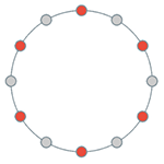
[2.1.2] A maximally even (ME) set is simply a distribution of a group of things over a limited amount of space, where the things are spread as evenly apart as possible. To visualize this, picture the familiar clock face. Each hour is numbered, and each number could be assigned to a chromatic pitch class. If you choose six notes from the chromatic scale, with the goal of maximal evenness, you would want to choose six notes each a whole step apart. On the clock face (here, abstracted into a collection of points around a circle), this is a selection of every other point (Example 1).
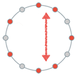
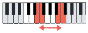
[2.1.3] Such a selection is a totally even distribution, with each selected item separated from the next by an equal amount. The diatonic set is not totally even, but instead a maximally even distribution of seven notes over the chromatic scale (written 7→12). This distribution cannot be totally even, because seven shares no common factors with twelve. So it is as even as possible, with the two anomalous half steps placed as far apart from each other as they can be (Example 2a). A different visualization shows this selection of seven notes out of one chromatic segment on a piano keyboard (Example 2b).
Example 2a. The pairs of adjacent red dots are as far apart as possible, as indicated by the red arrow
(click to enlarge) | Example 2b. On the keyboard, the pairs of adjacent white keys are as far apart as possible (for a white-note collection)
(click to enlarge) |
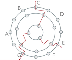
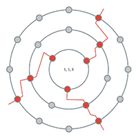
[2.1.4] Another familiar maximally even distribution is a triad within a diatonic key. Instead of a clock face with twelve parts, picture a clock face of only seven parts, where each of those parts represents one of the seven diatonic notes. Selecting three notes as far apart as possible (a maximally even distribution of 3→7), Example 3 shows the C+ triad as one possible result. The difference between 7→12 and 3→7 is subtle: In the former, the circle is divided into 12 equal parts, just like 12-note equal temperament equally divides the octave. Because of this, 7→12 gives us a ME distribution that is easily and accurately associated with chromatic space. In the latter, the circle is divided into 7 equal parts. A diatonic collection is not made of an equal division of the octave into 7 parts, though we can conceive of this evenly-spaced representation as a scale-step space. When the two independent diagrams are joined, the image of the scale-step space in 7→12 yields an explicit diatonic key, and the image of 3→7 yields an explicit triad within that key.(2) A triad, then, is a maximally even distribution over a diatonic subset, and to get this diatonic subset, we use the results of 7→12 to constrain the results of 3→7. This is more conventionally notated as 3→7→12, and is known as an iterated ME set (Example 4).
Example 3. A C+ triad as a maximally even distribution of three notes in a 7-note collection
(click to enlarge) | Example 4. 7→12 and 3→7 combine to visually portray a 2nd-order maximally even set
(click to watch video) |

Determining maximal evenness using FiPS
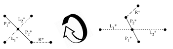
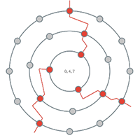
[2.2.1] Moving beyond the basic notion of “as even as possible,” we use FiPS as a geometric method to determine any ME distribution (including iterated ME distributions). FiPS relies on a minimum of two rings, each with some number of points evenly placed around it. The most interior ring is called the beacon, and all other rings are called filters. The beacon emits a beam from each of its points, and when the beam encounters a filter, the beam follows these simple rules (see Example 4 for an animated reference):
- If the beam directly aligns with a point on the filter, it will pass through that point.
- If the beam does not directly align with a point on the filter, it will travel counterclockwise along the wall of the filter until it does encounter a point to pass through.
- The beam always leaves from a point in a direction normal to that point. This means that, after the beam passes through a point on a filter, the direction of the beam will be altered. It will always point directly outwards from the filter. For clarity in the animations, you can always see this change in beam direction prior to the beam reaching the next point. A beam will start normal to the beacon, and split in the middle to become normal to the point through which it will pass on the next filter.
Example 5. Seven pentatonic collections as part of a 5→12 FiPS configuration
(click to watch video)
[2.2.2] Some familiar ME sets in the chromatic universe are the pentatonic, diatonic, and octatonic collections. Examples 5–7 show each of these collections, respectively, as determined by Filtered Point-Symmetry. Each animation shows an interior ring of the given cardinality rotating within an exterior ring of cardinality 12. The rotations cause the active holes on the chromatic ring to change based on the rules given above. In the case of the pentatonic and diatonic collections, you will see each one of the 12 collections; in the case of the octatonic collection, you will see the three distinct collections.
Example 6. Seven diatonic collections as part of a 7→12 FiPS configuration
(click to watch video) | Example 7. Three octatonic collections as part of an 8→12 FiPS configuration
(click to watch video) |
[2.2.3] Example 8 shows 3→7 behaving similarly to the prior animations. It is slightly more abstract than the prior material, in that (as in Example 4) we are imaging that the 7-hole ring corresponds to some generic diatonic collection. It could be C major,
Example 8. Seven implicitly diatonic chords as part of a 3→7 FiPS configuration
(click to watch video) | Example 9. Seven explicitly diatonic chords as part of a 3→7→12 FiPS configuration
(click to watch video) |
Correspondence with the J function
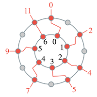
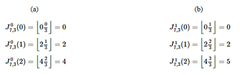
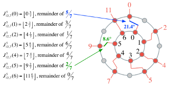
[2.3.1] The J function, defined by Clough and Douthett (1991) in their seminal article “Maximally Even Sets” is given as $$ J_{c,d}^m\left( k \right) = \left\lfloor {\tfrac{{ck + m}}{d}} \right\rfloor $$ where $0 \leqslant k \leqslant d-1$, such that an ME set with these parameters is $$ J_{c,d}^m=J_{c,d}^m(\mathbb{Z}_d)=\{ J_{c,d}^m(k) \}^{d-1}_{k=0} $$ The $J$ function was first used in reference to the diatonic collection, and the variables are named in deference to that use case: $c$ referred to the cardinality of the chromatic collection (12) and $d$ referred to the cardinality of the diatonic collection (7). More generally, we can think of $c$ referring to the cardinality of the container, and $d$ referring to the cardinality of the distributed set. (In a 7→12 distribution, $c=12$ and $d=7$. In a 3→7 distribution, $c=7$ and $d=3$.) The other value, $m$, is an offset value that I will explain shortly, but for now it is sufficient to notice that $m$ is used in conjunction with the pair of values $c$ and $d$. For the current example, we are going to arbitrarily assign this offset $m$ a value of 5. The value $k$ is the element in the distributed set that one is curious about. For instance, in our 7→12 distribution, we want to know to which of the 12 chromatic pitches each of the seven elements ${0, 1, 2, 3, 4, 5, 6}$ goes. The right side of the equation is wrapped in brackets with feet; these brackets represent a quantization function known as the floor function, which truncates any fractional value from a number to make it an integer.(3) The ME algorithm will step through all of these values of k with the $J$ function (usually written $J_{c,d}^m$), the result of which is the C-major diatonic collection: $$\eqalign{ & J_{12,7}^5(0) = \left\lfloor {\tfrac{{12 \bullet 0 + 5}}{7}} \right\rfloor = \left\lfloor {\tfrac{5}{7}} \right\rfloor = \left\lfloor {0\tfrac{5}{7}} \right\rfloor = 0 \cr & J_{12,7}^5(1) = \left\lfloor {\tfrac{{12 \bullet 1 + 5}}{7}} \right\rfloor = \left\lfloor {\tfrac{{17}}{7}} \right\rfloor = \left\lfloor {2\tfrac{3}{7}} \right\rfloor = 2 \cr & J_{12,7}^5(2) = \left\lfloor {\tfrac{{12 \bullet 2 + 5}}{7}} \right\rfloor = \left\lfloor {\tfrac{{29}}{7}} \right\rfloor = \left\lfloor {4\tfrac{1}{7}} \right\rfloor = 4 \cr & J_{12,7}^5(3) = \left\lfloor {\tfrac{{12 \bullet 3 + 5}}{7}} \right\rfloor = \left\lfloor {\tfrac{{41}}{7}} \right\rfloor = \left\lfloor {5\tfrac{6}{7}} \right\rfloor = 5 \cr & J_{12,7}^5(4) = \left\lfloor {\tfrac{{12 \bullet 4 + 5}}{7}} \right\rfloor = \left\lfloor {\tfrac{{53}}{7}} \right\rfloor = \left\lfloor {7\tfrac{4}{7}} \right\rfloor = 7 \cr & J_{12,7}^5(5) = \left\lfloor {\tfrac{{12 \bullet 5 + 5}}{7}} \right\rfloor = \left\lfloor {\tfrac{{65}}{7}} \right\rfloor = \left\lfloor {9\tfrac{2}{7}} \right\rfloor = 9 \cr & J_{12,7}^5(6) = \left\lfloor {\tfrac{{12 \bullet 6 + 5}}{7}} \right\rfloor = \left\lfloor {\tfrac{{77}}{7}} \right\rfloor = \left\lfloor {11\tfrac{0}{7}} \right\rfloor = 11 \cr} .$$
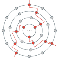
Example 10. A 7→12 maximally even distribution, with connections between indices explicitly traced
(click to enlarge)
[2.3.2] When we revisit the FiPS representation of this distribution, we can associate each point on the 7-beacon with the corresponding point on the 12-filter and see that the resulting set is identical. Example 10 shows the values of $k$ in black, next to corresponding points on the interior ring, and shows the resulting values of $J(k)$ in red, next to corresponding points on the exterior ring. Additionally, we can see that point 6 on the 7-beacon has a beam that passes directly through point 11 on the 12-filter, and all other beams travel counter-clockwise to some extent before passing through a point on the 12-filter. The proportion of counter-clockwise movement on the 12-filter (or lack thereof) corresponds precisely to the fractional remainder for each $k$ in the list, and the distinctiveness of the straight beam is due precisely to the equivalence in the equation $J_{12,7}^5(6) = \left\lfloor {11\tfrac{0}{7}} \right\rfloor = 11\tfrac{0}{7}$, where the floor function is unnecessary. In other words, counter-clockwise movement to the nearest point is the geometric analogue of the floor function.
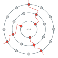
[2.3.3] Just as $J_{12,7}^5$ describes Example 10, $J_{7,3}^0$ describes the values seen in Example 3 and at the starting position of Example 8: $$\eqalign{ & J_{7,3}^0(0) = \left\lfloor {\tfrac{{7 \bullet 0 + 0}}{3}} \right\rfloor = \left\lfloor {\tfrac{0}{3}} \right\rfloor = \left\lfloor {0\tfrac{0}{3}} \right\rfloor = 0 \cr & J_{7,3}^0(1) = \left\lfloor {\tfrac{{7 \bullet 1 + 0}}{3}} \right\rfloor = \left\lfloor {\tfrac{7}{3}} \right\rfloor = \left\lfloor {2\tfrac{1}{3}} \right\rfloor = 2 \cr & J_{7,3}^0(2) = \left\lfloor {\tfrac{{7 \bullet 2 + 0}}{3}} \right\rfloor = \left\lfloor {\tfrac{{14}}{3}} \right\rfloor = \left\lfloor {4\tfrac{2}{3}} \right\rfloor = 4 \cr} .$$
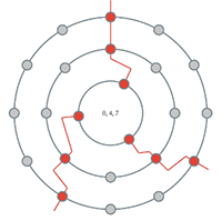
[2.3.4] Clough, Cuciurean, and Douthett (1997) formally define an iterated ME set as $$ J^{m_1, m_2, \dots, m_n}_{d_0, d_1, d_2, \dots, d_n} = J^{m_1, m_2, \dots, m_n}_{d_0, d_1, d_2, \dots, d_n}(\mathbb{Z}_{d_n})=\left\{J^{m_1, m_2, \dots, m_n}_{d_0, d_1, d_2, \dots, d_n}(k)\right\}_{k=0}^{d_n-1} $$ where $$ J^{m_1, m_2, \dots, m_n}_{d_0, d_1, d_2, \dots, d_n} \left( k \right) = J_{d_0, d_1}^{m_1} \left( J_{d_1, d_2}^{m_2} \left( J_{d_2, d_3}^{m_3} \left( \dots J_{d_{n-1},d_n} \left( k \right) \right) \right) \right) $$ In this representation, the sequence of subscript values represents the chain of distributions from right to left, such that the subscript for a 3→7→12 distribution would appear as $J_{12,7,3}$. The still-to-be-discussed superscript $m$ values are associated with pairs of subscript values, such that $m_1$ is associated with $d_0$ and $d_1$, and $m_2$ is associated with $d_1$ and $d_2$. An iterated maximally even set represented as $J_{12,7,3}^{5,0}$ is evaluated with superscripts and subscripts from right to left. The first evaluation is $J_{7,3}^0$, and the next is $J_{12,7}^5$. Unlike the previous rendition of $J_{12,7}^5$, however, only the results of the previously-derived ME set are used as values for $k$. The result of this is a C+ triad ${0,4,7}$, as shown in the following, connected pair of equations:

Changes over time
[2.4.1] The value $m$ in the $J$ function is called the mode index, and is most appropriately named in the context of the 7→12 distribution. In $J_{12,7}^m$, when $m = 0$, the result is the
Example 11. (a) A calculation of
(click to enlarge)
[2.4.2] Returning once more to Example 9, you see a 3→7→12 FiPS configuration with the 3-beacon continuously rotating clockwise. As it rotates, the output of the system is the repeating series <C+, A−, F+, D−, B°, G+, E−>. This series involves all the ME triads within C major, where the change between triads preserves as many common tones as possible.(4) When you rotate the 3-beacon clockwise in 3→7→12, you are algebraicly using $J_{12,7,3}^{m_1, m_2}$, holding $m_1$ constant at $m_1=5$ (for C major), and increasing the value of $m_2$ over time. Focusing on the algebra for just the first iteration, $J_{7,3}^{m_2}$: as $m_2$ increases, the result set is altered when $ \lfloor m_2 \rfloor = 0$ becomes $\lfloor m_2 \rfloor =1$. Explicitly, when $\lfloor m_2 \rfloor =1$, $1/d$ (in this case $1/3$) is added to each of the values of ${\tfrac{ck}{d}}$ prior to the floor function being applied. As shown in Example 11, the addition of $1/3$ to each value changes the diatonic set from $\{0, 2, 4\}_{mod\ 7}$ to $\{0, 2, 5\}_{mod\ 7}$, meaning that the fifth element of a diatonic collection (at value 4) is exchanged for the sixth (at value 5); in C major (assuming 0 is pitch-class C), this constitutes a change from pc G to pc A.
Example 12. There is an equal distance of 30° (30° = 360/12) between points on the outer ring. Each remainder corresponds to the distance between the beam of the beacon and the distance it must travel counter-clockwise to reach an evenly-spaced hole on the outer ring.
(click to enlarge)
[2.4.3] Because the fractional remainders are different for each value of $k$ in Example 11, changing the value of $m_1$ will never result in more than one output value changing at a time. No more than one note will change at a time whenever the cardinality of the distributed set shares no common factors with the cardinality of the set into which it is distributed (such a relationship of cardinalities is called coprime, represented by the symbol $ \bot $). 3 and 7 are coprime, and 7 and 12 are coprime, or $3 \bot 7$ and $7 \bot 12$. Returning to the FiPS visualization, Example 12 shows a 7→12 distribution in which the remainders are identified for each equation. Because 7 and 12 are coprime, each remainder is unique, and each unique remainder corresponds to a unique number of degrees between the beam from the beacon and the distance that must be traveled counter-clockwise to a filter hole. When the beacon rotates continuously, the distances remain unique for each of the beams, such that only one value changes at a time.
[2.4.4] In the next section, we are going to look at more distributions. We will expand our study to the octatonic and enneatonic collections, and explore analytical spaces that allow us to easily determine the result for rings in any position, even when both rings are moving simultaneously.
Configuration Spaces and Scalar Contexts
The neo-Riemannian Tonnetz
Example 13. A 3→8→12 configuration in which a C- triad is the result

(click to enlarge)
[3.1.1] The most ubiquitous geometry for transformations between trichords is the neo-Riemannian Tonnetz. The common triad cycles may all be generated using a few relatively simple 3-ring FiPS configurations, and the relationship between the models creates the possibility of a different perspective on the capabilities of this geometric space.
[3.1.2] To begin, let’s examine a FiPS configuration of 3→8→12 (Example 13). The outermost two rings, 8→12, work together to select a particular octatonic collection, as in Example 7, and the two innermost rings, 3→8, select a 3-note ME subset of that particular octatonic. Because the beacon selects a subset of the octatonic provided by the outermost rings, dashed lines have been used in this figure to indicate the inactive members of the 8→12 distribution. (As opposed to the examples in the previous section, 8 and 12 are not coprime. The impact of this difference is explored in the next section, “Parsimony and Displacement.”)
Example 14. A 3→8→12 configuration in which all members of the 01-octatonic are realized
(click to watch video)
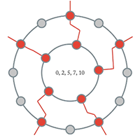
[3.1.3] In Example 14, as in Example 13, the 01-octatonic is selected. Here, we see the beacon rotate to incrementally change the selection of the maximally even subset. The harmonic output of Example 14 is <$\{0, 3, 7\}$, $\{0, 4, 7\}$, $\{0, 4, 9\}$, $\{1, 4, 9\}$, $\{1, 6, 9\}$, $\{1, 6, 10\}$, $\{3, 6, 10\}$, $\{3, 7, 10\}$, $\{3, 7, 0\}$>, where the last set is the same as the first, such that this forms an eight-chord cycle. All of these chords belong to the same set class, because all 3-note ME subsets of an octatonic collection belong to the set class of major and minor triads (0, 3, 7).
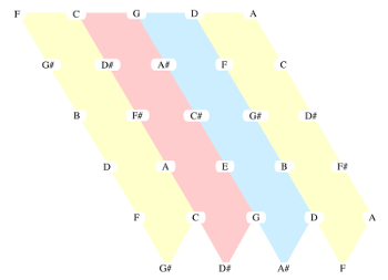
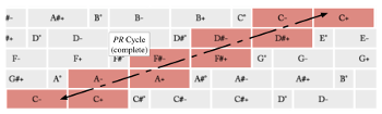
[3.1.4] The Tonnetz bears a strong resemblance to this octatonically configured example; the output of Example 14 is exactly the neo-Riemannian $PR$ (octatonic) cycle. Example 15 highlights each of the three octatonic corridors in the Tonnetz, where such a corridor is bounded on either side by a diagonal line of minor-third-related pitch-classes. The light red octatonic corridor of Example 15 contains exactly the same triads as Example 14; it is showing us the eight triads that are (uniquely) subsets of the 0,1-octatonic.
Example 15. The neo-Riemannian Tonnetz, with highlighted octatonic corridors
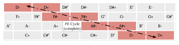
(click to enlarge) | Example 16. The neo-Riemannian Tonnetz with highlighted octatonic corridors, and a PL cycle following a path within and then out into each corridor
(click to enlarge) |
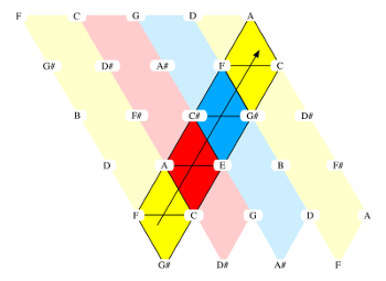
[3.1.5] If we continue to think of the Tonnetz as a collection of three octatonic corridors, each containing a unique slice of the 24 possible triads, then we can conceive of other common neo-Riemannian cycles as patterns that move within and between these three corridors. For example, the $PL$ (hexatonic) cycle can be thought of as a cycle that first moves within an octatonic corridor (via $P$) and then out into an adjacent corridor (via $L$). Example 16 shows such a cycle on the Tonnetz. Every triad in the cycle is colored according to its octatonic corridor. Each pair of similarly-colored triads are $P$-related; for instance, A− and A+ are both situated in the red (0,1) octatonic. Instead of continuing an octatonic cycle after A+, the $PL$ cycle has us step out into the blue octatonic corridor.
Example 17. A 3→8→12 configuration in which a PL cycle is realized, in the manner of Example 16
(click to watch video)
[3.1.6] Such a move—within and then out into—is precisely the manner in which we can conceive of this gesture using FiPS. Example 14 shows the isolated rotation of a 3-hole beacon (where the 8-hole filter is immobile), and Example 7 shows the isolated rotation of the 8-hole filter, which changes the octatonic collection. Example 17 shows both events happening synchronously: both the beacon and the 8-hole filter are rotating, causing chord-within-collection and chord-out-into-collection changes to occur, over the same chord path as indicated in Example 16. Similar to the $PL$ cycle, the $RL$ cycle—which traverses all 24 major and minor triads—also executes an alternating chain of within and out into actions.
[3.1.7] You may notice a discrepancy between the description above and the visualization, namely that the 3-hole beacon appears stationary. Let me explain this appearance of non-motion in greater detail, which will also serve to clarify exactly how we visualize the process of iteration in the $J$ function. As the 8-hole filter rotates, it takes the 3-hole beacon along for the ride, as though the 3-hole beacon were a hubcap attached to a tire. If the 3-hole beacon had no change in its associated value of $m$ over time, we would see it rotating in the visualization and maintaining its position with respect to the 8-hole filter. To appear stationary, the 3-hole beacon rotates at a rate of change opposite that imposed by the 8-hole filter, as though it’s on a treadmill or hamster wheel doing just enough work to stay in place. So, although it appears stationary, the value of $m_2$ (for the 3-hole/8-hole pairing) increases over time, causing a clockwise motion that counters the decreasing value of $m_1$ for the 8-hole/12-hole pairing.
Example 18. A 3→8→12 configuration space
(click to enlarge)
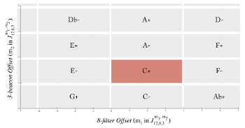
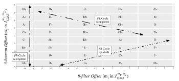
[3.1.8] The iterated $J$ function $ J^{m_1, m_2, \dots, m_n}_{d_0, d_1, d_2, \dots, d_n} $ is predictable: by putting in a certain set of values for $d_{n-1}$, $d_{n}$, and $m_n$, the resulting ME set is a single, consistent result. FiPS, in modeling the $J$ function, shares this predictability: for any combination of ring cardinalities and rotational offsets, there is a single, consistent result. This property allows us to gather information about all possible outcomes for any set of ring cardinalities. Example 18 is a configuration space—a model of all possible outcomes for a range of ring positions in a 3→8→12 configuration. This could be represented as an iterated $J$ function where $d_0=12$, $d_1=8$, and $d_2=3$. The numbers along the axes in Example 18 indicate the values of $m_n$ in the $J$ function ($m_1$ along the x-axis, and $m_2$ along the y axis). For a moment, look closely at the C+ triad highlighted in red. For this triad, the values of $m_1$ along the y-axis fall into the range $[1, 2)$. The values of $m_1$ along the x-axis fall into the range $[0, 4)$. In this particular configuration, as indicated clearly in the configuration space, any combination of values in those ranges will yield a C+ triad.
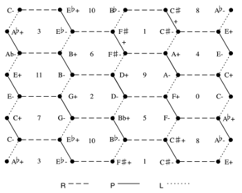
[3.1.9] Jack Douthett and Peter Steinbach (1998) describe a Chicken-Wire Torus as the geometric dual of the Tonnetz. Instead of each node representing a pitch-class, each node instead represents a triad. (Example 19) Chord-for-chord and transformation-for-transformation, the Chicken-Wire Torus maps onto the 3→8→12 configuration space (Example 20). This isomorphism is significant: all parsimonious neo-Riemannian triadic transformations are modeled—completely and with nothing extraneous—in a configuration involving maximally even trichords within octatonic collections.
Example 19. Douthett and Steinbach’s (1998) Chicken-Wire Torus
(click to enlarge) | Example 20. A portion of a 3→8→12 configuration space, with a matching portion of the Chicken-Wire Torus overlaid to demonstrate the isomorphism
(click to enlarge) |
[3.1.10] In addition to the Chicken-Wire Torus, Douthett and Steinbach (1998) present another diagram called the Towers Torus, which models a particular set of tetrachordal transformations that bears some similarity to the triadic $LPR$ group. Following from the Tonnetz isomorphism, we find a similar match in a 4→9→12 FiPS configuration space (Example 21). Because the original Towers Torus diagram and the diagrams that follow do not correspond without some rotation and stretching, Example 22 is provided to demonstrate the adjustments made to the shape—but not the substance—of the original diagram.(5)
Example 21. A portion of a 4→9→12 configuration space, with a matching portion of the Towers Torus overlaid to demonstrate the isomorphism
(click to enlarge) | Example 22. On the left, the original key to Towers Torus from Douthett and Steinbach. On the right, a rotated and slightly stretched version of the key that reflects the altered positioning of the diagram when overlaid on the 4→9→12 configuration space
(click to enlarge) |
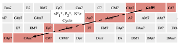
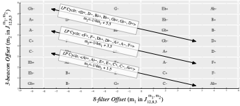
[3.1.11] The next section of this study will dive deeply into considerations of voice-leading parsimony, including a discussion of transformational labels such as $L$, $P$, and $R$, and Douthett and Steinbach’s proposed modifications to these labels for the tetrachordal Towers Torus. For now, I’d like to simply draw attention to the fact that the 3→8→12 configuration space can model common parsimonious trichord cycles (Example 23), and the 4→9→12 configuration space can model parsimonious tetrachord cycles (Example 24). The modeling itself is due to the isomorphism of the particular configuration space with a particular torus. A more interesting facet is the strong visual parallel between the spaces and labeled lines in Examples 23 and 24. Even though the spaces are different, the lines represent similarly endless walks through harmonic cycles. Example 25 contains an animation of the <$P_1*, P_2*, R*$> cycle (a visual analogue to the neo-Riemannian $PR$ cycle of Example 14). Example 26 contains an animation of the <$P_2*, L_2*$> cycle, a clear visual analogue to the neo-Riemannian PL cycle of Example 17.
Example 23. A 3→8→12; configuration space with neo-Riemannian cycles identified
(click to enlarge) | Example 24. A 4→9→12 configuration space with Towers Torus cycles identified
(click to enlarge) |
Example 25. The <P1*, P2*, R*> cycle identified in Example 24
(click to watch video) | Example 26. The <P2*, L2*> cycle identified in Example 24
(click to watch video) |

Diatonic Configurations
Example 27. A parsimonious cycle of diatonic trichords in C major
(click to watch video)
[3.2.1] To be sure, the isomorphisms above show us something about how voice-leading parsimony corresponds to iterated maximally even sets, but we would be in error if we said that all neo-Riemannian triadic transformations occur only when the music takes an octatonic turn, or that we are necessarily in an enneatonic passage when there are parsimonious connections between tetrachords. Let’s put ourselves in a diatonic mindset, using a 3→7→12 FiPS configuration. As demonstrated in Example 6 and Example 8, the position of the 7-filter determines the diatonic collection, and the position of the 3-beacon selects a maximally even 3-note subset of that particular diatonic collection. If only the 3-beacon rotates, as in Example 9 (which is in
Example 28. A 3→7→12 configuration space

(click to enlarge)
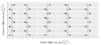
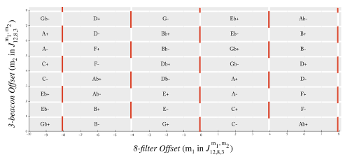
[3.2.2] Example 28 gives a 3→7→12 configuration space, where each of the 36 major, minor, and diminished ME diatonic triads is represented. Because these diatonic triads are a superset of the 24 ME octatonic triads, the conventional neo-Riemannian cycles can be modeled in diatonic space. Examples 29, 30, and 31 each highlight one of the three previously-discussed neo-Riemannian cycles ($PR$, $PL$, and $LR$, respectively). Of particular importance is the fact that although these are the same harmonies, these cycles are not identical to those inscribed in the 3→8→12 space.
Example 29. A PR cycle in a 3→7→12 configuration space
(click to enlarge) | Example 30. A PL cycle in a 3→7→12 configuration space
(click to enlarge) |
Example 31. An LR cycle in a 3→7→12 configuration space
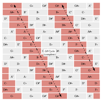
(click to enlarge)
[3.2.3] In our octatonic configuration, we conceived of $PR$ as something that occurs entirely within a single octatonic collection (a corridor in the Tonnetz). This cycle of chords cannot take place within a single diatonic key. FiPS suggests that we might instead describe this cycle, in diatonic space, as an intra-key transformation from a major tonic to its relative minor, followed by a change of diatonic key, where the triad is eventually impacted by a change to the key signature itself. Imagine yourself at the piano with a C+ triad. You might be in F major, C major, or G major. An R transformation takes you to an A− triad, and you may still be in any of the three aforementioned keys. But whatever key you do happen to be in, imagine that the key signature is steadily increasing sharp-wise, such that you eventually find yourself in the key of D major. At this moment in time, the C in your A− triad may not persist, forcing you to an A+ triad (the P transformation). This alteration of R and P continues until the cycle is complete.
Example 32. An LR cycle in a 3→5→12 configuration space
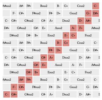
(click to enlarge)
[3.2.4] The $PR$ cycle in the diatonic is more similar to the octatonic $PL$ and $LR$ cycles, in that it consists of inter- and intra-key chord changes. Although we will not necessarily hear a number of key changes in a neo-Riemannian triadic cycle of any length, we should consistently take into consideration the scalar context in which such chord progressions occur: are we listening to music that seems more outside of tonality, in some grounded octatonic region, or are we listening to music that moves more tonally and sequentially in a non-grounded-but-tonal manner? One final note on the neo-Riemannian triadic progressions: consider as well the 3→5→12 configuration space given in Example 32. Highlighted is an $LR$ cycle, consisting of intra-pentatonic-key $R$ and inter-pentatonic-key $L$ transformations. Although parsimonious $PL$ and $PR$ cycles are not possible in a pentatonic collection, the presence of $LR$ serves as an additional indicator that chords alone do not provide complete information for these non-tonal transformational progressions. Further, the sus2 (or sus4) chords appearing in the example are maximally even trichords in a pentatonic collection. In a musically pentatonic world, this set class occupies the same distributional status as a triad, and not the suspension-to-a-triad status it would have when used in a diatonic collection.
Example 33. A 4→7→12 configuration space
(click to enlarge)
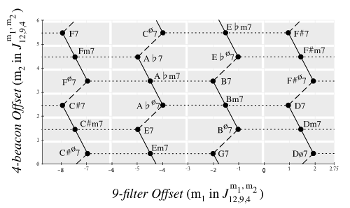
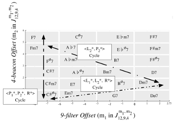
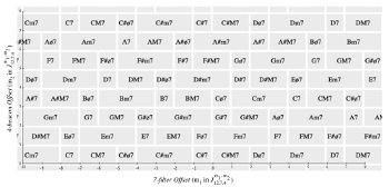
[3.2.5] Just as the diatonic trichords superset the ME octatonic trichords represented by the Tonnetz, diatonic tetrachords superset the ME enneatonic tetrachords represented by the Towers Torus. Example 33 gives a 4→7→12 configuration space, and Examples 34 and 35 trace two parsimonious voice-leading paths through that space, in cycles that are chord-equivalent (though not quality-equivalent) to their Towers Torus counterparts from Example 24. Example 36 highlights the chords of the <$L_1*, L_2*, R*$> cycle shown in Example 24, but Example 36 fails to replicate this cycle: a straight line cannot be drawn that connects only the Towers Torus chords, and in Example 36 you can see that the line intersects a number of major-seventh chords (highlighted in yellow).
Example 34. A <P1*, P2*, R*> cycle in a 4→7→12 configuration space
(click to enlarge) | Example 35. An <L2*, P2*> cycle in a 4→7→12 configuration spac
(click to enlarge) |
Example 36. A cycle in a 4→7→12 configuration space that augments an <L1*, L2*, R*> cycle
(click to enlarge)
[3.2.6] In Example 36, the inability to draw a straight line through the <$L1*, L2*, R*$> cycle shows that, in 4→7→12, a cycle involving only those transformations is of a different nature than a cycle that can be represented by a straight line. To properly address this example in detail, we need a coherent and concrete understanding of parsimony, as well as language to distinguish those cycles that can be represented by straight lines from those that cannot. The next section takes on these tasks.
Parsimony and Displacement
Parsimony (Scalar and Chromatic)
[4.1.1] We might think of “voice-leading parsimony” as reasonably well-defined, considering the decades it has appeared in music-theoretical literature. Yet parsimony has a multitude of definitions, and existing literature has examples with varying parameters. In the first part of this section, I am going to step back from configuration spaces to capture the current definitions of parsimony, highlight some key concepts, and use scale theory to help make our conception of parsimony more concrete. At the very least, clarity around the term will prove useful for the purposes of the current discussion. In the second part of this section, I will return to configuration spaces and propose a more precise way of characterizing displacement operations between chords in a scalar context. In the final part of this section, I will look at uniform cycles in scalar contexts, and at the varying degrees of parsimony in those cycles.
[4.1.2] The imprecision in the term “voice-leading parsimony” has led to an array of descriptions and rule-sets that, while similar, are not consistent.(7) For instance, all theories of voice-leading parsimony are concerned with some manner of minimal change, where minimal change is evocative of a small quantity of pitches changing by a limited interval. Usually, but not always, the small quantity of pitches is “one pitch,” though Childs 1998 focuses on transformations between dominant and half-diminished seventh chords (sc4-27) where two pcs change in each transformation, and Douthett and Steinbach 1998 create $p_{m,n}$ notation to indicate a change between chords involving $m$ notes changing by half step and $n$ notes changing by whole step, where either of those values can be greater than one. What constitutes a limited interval is similarly without concensus, though agreement is often found in a measure of 1 and/or 2 semitones.(8) As in neo-Riemannian theory, 2-semitone parsimonious changes often occur in discussions involving similarly-even or identical set classes; 1-semitone parsimonious changes seem to be preferred in approaches that deal with a wider array of set classes, such as Cohn 2003 and Straus 2005.(9) To summarize the first two points, and add a third observation on set class:
- when a voice moves by a limited interval, that interval is usually 1 or 2 semitones
- when a small quantity of pitches change, usually that small quantity is 1; and
- parsimonious models seem to either follow specific sets within a limited family of set classes that have similar (and high) evenness, or they follow a broad family of set classes and are primarily concerned with smooth changes between sets of different types.(10)
[4.1.3] Let’s now be more specific about the first of these points, where a voice moves by a limited interval of 1 or 2 semitones. As noted above, in models that deal with a multitude of set classes, there seems to consistently be a 1-semitone limit, and intervals of 2 semitones surface when there is a discussion of chords or a (related) discussion of evenness-preserving changes. The classic neo-Riemannian example of Cohn 1997 serves as an excellent model for this, consider Example 20, which shows the isomorphism of the neo-Riemannian model of trichords and the 3→8→12 configuration space. These spaces are notably distinct—the latter represents both the chords and the collections from which they are derived, whereas the Tonnetz makes no inference about the octatonic—yet it is the isomorphism that explains why the neo-Riemannian model is drawn to 1- and 2-semitone changes: an octatonic space has scalar step sizes of exactly 1 and 2 semitones. In fact, scalar context provides such a consistent, universal justification for the varied step sizes discussed in the literature on parsimony that we might state the following:
Trait 1: When a voice moves by a limited interval, that interval is a single scale step.
[4.1.4] The chromatic sizes of a single scale step are determined by taking the floor and ceiling of the ratio of the cardinality of the chromatic set to the cardinality of the scale. (This will be true for any maximally even collection, since a defining property of maximal evenness is for every generic interval to exist in one integer size or two consecutive integer sizes.) In the case of the whole tone scale, a step will consistently be 2 semitones, since $\lfloor12/6\rfloor = \lceil12/6\rceil = 2$. And in the case of the pentatonic, the step sizes will be 2 or 3 semitones, since $\lfloor{12/5}\rfloor=2$ and $\lceil{12/5}\rceil=3$. In all other scales that are part of the chromatic universe—those we study most when looking at parsimony between chords—a scale step will consist of 1 or 2 semitones, as practice has already led us to observe. The chromatic is a special case, in the sense that one does not have a chromatic scale distributed within the chromatic universe, though if one did, it would always yield a 1-semitone step, since $12/12 = 1.$ In practice, the analyses that are dealing with many set classes are operating in the chromatic universe, and are constrained to a 1-semitone step precisely because there is no scale that could apply to the broad selection of set classes being examined—a point we will return to shortly.
[4.1.5] The second item listed above is that only a small number of pitches are changed in a parsimonious transformation. As noted, that small number is usually one, but with exceptions. I recently posed the following scenario to my colleagues: “We are likely to agree that the C-major diatonic is parsimoniously related to G major and F major. I would make the same case for the relationship of the three octatonic collections, for when I look at the corridors on the neo-Riemannian Tonnetz, the close-as-possible relationship of the collections jumps out to me as similar to how we see closely-related diatonic keys. Do you think of the octatonic collections as parsimoniously related?” The spontaneous reaction—one with which I fully agree—is that yes, the relationship is parsimonious. The problem, of course, is that each octatonic collection has a four-note difference with any other. Instead of calling this un-parsimonious because of the quantity of notes changing, the following reasoning seems to be broadly inclusive of existing discussions of parsimonious transformations, along with the octatonic collection scenario noted here:
Trait 2: When a small quantity of pitches change, that quantity is the minimum gcd as determined by a consideration of collection and scale size, where the cardinality of the smallest collection is greater than 2.
[4.1.6] To apply this reasoning to changes between closely-related collections, we take $\gcd(12, 7)=1$ to see that a parsimonious transformation between closely-related diatonic keys will involve the change of a single pitch. Applied to octatonic collections, $\gcd(12, 8)=4$ would be taken to mean that a parsimonious transformation between octatonic collections involves a four-note change. But this latter point does not mean that four-note changes are parsimonious outside of a consideration of the octatonic collections as a whole. Triads in the octatonic present a series of relationships such that, for 3→8→12, we calculate $\min(\gcd(12, 8), \gcd(8,3))=1$ and use this to say that a parsimonious transformation between triads in octatonic collections involve single pitch changes. In 4→6→12, I would expect a parsimonious transformation to involve a change of two notes, each by whole step. I expect two notes to change because $\min({\gcd(12,6), \gcd(6,4)})=\min(6, 2)=2$ (and I expect those pitches to change by whole step because $\lfloor12/6\rfloor = \lceil12/6\rceil = 2$). More generally, assuming a distribution that uses $d_n$ following the notation of the $J$ function, the number of notes changing in a parsimonious transformation is $\min(\gcd(d_0, d_1), \gcd(d_1, d_2), \ldots , \gcd(d_{n-1}, d_n))$.(11)
[4.1.7] Finally, I would address the observation that appears third in the list above, regarding the chord relationships that are examined in studies of voice-leading parsimony. For studies that limit themselves to discussion of a few set classes, set class preservation is a prominent concern. It is neither a consistent nor universal concern in discussions of parsimony—in fact, it is precisely the relaxation of concerns about set class preservation (towards greater evenness) that leads Douthett and Steinbach 1998 to form Power Towers from the three OctaTowers—but the existence of this concern should be examined. In “General Equal-Tempered Harmony,” Ian Quinn (2006 and 2007) demonstrates how the discrete Fourier transform can be used as a measure of evenness for different set classes. This work is expanded by Callender, Quinn, and Tymozcko (2008) in their generalized voice-leading spaces, and in these spaces chords of similar evenness sit in close proximity. If one envisions a totally even chord in voice-leading space encased in a small sphere, then all the chords that are nearly even can be included in a slightly-larger sphere, such that all maximally-even chords sit in very close proximity to one another. Because of this, it stands to reason that nearly-even set classes are commonly the focus of parsimonious transformation studies (one is able to more efficiently visit all nearly-even chords from a series of parsimonious moves than one could efficiently visit all similar less-even chords). Still, there are at least two distinct approaches to parsimony: a sort of chromatic parsimony that is concerned with a multitude of set classes (or even all set classes of a particular size), and another sort of parsimony that seems like it can be clarified with scale theory. For this latter type, I would say that there even exists a special type of parsimonious transformation, $p_e$, which preserves evenness between chords. The neo-Riemannian transformations would fall into this special category. And, with the use of scales, the parsimonious relationship of G+ and B° is particularly interesting because it is $p_e$ in the diatonic, and only $p$ in the octatonic.
Displacement Operations
[4.2.1] As noted above, the fact that the changes G+→E− and G+→B° may both be parsimonious changes of harmony does not tell a complete story, especially with respect to the collections in which those changes occur. Specifically, pitch-class equivalence alone does not create chord equivalence outside of the chromatic set.(12) The prior discussion of diatonic configurations goes into great detail on the distinctions between neo-Riemannian operations in various configuration spaces, and G+→B° is particularly attention-grabbing in that, while it might represent an intra-key diatonic transformation in 3→7→12, in 3→8→12 it is not an evenness-preserving change, and it is a change that moves from within an octatonic collection to a space between octatonic collections. Returning to the example from the top of this section, we see another related problem of specificity: $\text{F} \!\! : \! \text{C}^7 \xrightarrow{\text L_2^*} \text{F} \!\! : \! \text{Am}^7$ and $\text{F} \!\! : \! \text C^7 \xrightarrow{\text L_2^*} \text G \!\! : \! \text{Am}^7$ are both parsimonious transformations, but the displacement involved in the latter could be characterized as a displacement that involves more work, since it includes a change of diatonic key. To make sense of the differences in chord changes involving identical sets of pitch classes, I propose the use of a displacement operation.
[4.2.2] A displacement operation $\delta$ is a translation in a specific configuration space, where that space is identified by subscript identical to that used in the $J$ function, $\delta_{d_0, d_1, d_2,\ldots,d_{n-1}, d_n}$. $\delta_{12,7,3}$, for instance, represents a displacement operation in the configuration space of diatonic triads, as in Example 28 above. A specific chord at a specific position in the configuration space is given by $\mathcal{K}$, where the position is identified by the $m_n$ values of the $J$ function, $\mathcal{K}_{m_1, m_2,\ldots,m_{n-1}, m_{n}}$. $\delta$ operates on these values of $m_n$ and takes as input the changes in $m_n$, so that $\delta(\Delta{m_1}, \Delta{m_2})_{12,7,3}$ would alter $m_1$ and $m_2$ of a chord $\mathcal{K}_{m_1,m_2}$. For instance, a displacement operation on the C+ harmony at $m_1=5, m_2=0$ is a displacement operation on the chord $\mathcal{K}_{5,0}$. A 1-unit clockwise rotation of a 3-hole beacon would be represented as $\delta(0, 1)_{12,7,3}$, and a 1-unit clockwise rotation of a 7-hole filter would be represented as $\delta(1, 0)_{12,7,3}$. A displacement involving a simultaneous clockwise rotation of the 7-hole filter and 3-hole beacon would be represented as $\delta(1, 1)_{12,7,3}$, and a counter-clockwise rotation of the 7-hole filter with a clockwise rotation of the 3-hole beacon would be represented as $\delta(-1, 1)_{12,7,3}$. Operations can be exponentiated for repetition, and also inverted, where inversion reverses the signs of all non-zero numbers: $\delta(0, 1)_{12,7,3}^{-1} = \delta(0, -1)_{12,7,3}$, and $\delta(-1, 1)_{12,7,3}^{-1} = \delta(1, -1)_{12,7,3}$. The application is straightforward: displacement values are added to the similarly-ordered $m$ values: $\mathcal{K}_{5,0}$ (C+, C:I) $\xrightarrow{\delta(1, 1)_{12,7,3}} \mathcal{K}_{5+1,0+1}$ (or $\mathcal{K}_{6,1}$, which is A−, G:ii).
[4.2.3] The values of $\Delta{m_n}$ can be any real number, and may or may not cause a change in harmony depending on the configuration space. Here are three distinct transformations using the same $\delta(2, 0)_{12,7,3}$ on different chords:
- $\mathcal{K}_{4,0}$ (C+, F:V) $\xrightarrow{\delta(2, 0)_{12,7,3}} \mathcal{K}_{7,0}$ (C+, G:IV)
- $\mathcal{K}_{5,0}$ (C+, C:I) $\xrightarrow{\delta(2, 0)_{12,7,3}} \mathcal{K}_{8,0}$ (
C♯ °, D:vii°) - $\mathcal{K}_{6,0}$ (C+, G:IV) $\xrightarrow{\delta(2, 0)_{12,7,3}} \mathcal{K}_{9,0}$ (C#-, A:iii)
In the first, the harmony does not change from C+; in the second, the harmony changes parsimoniously to
[4.2.4] A contextual shorthand for the displacement operation is $\delta^*$. $\delta^*$ guarantees a non-$T_0$ result, such that $\delta^*$ applied to a chord in a configuration space is always changed, regardless of how large or small a translation was required to cause the change. The values of $m_n$ in $d^*$ are accordingly restricted to the ternary set {-1, 0, 1}, where 0 indicates no change, 1 indicates a change caused by a clockwise rotation, and -1 indicates a change caused by a counter-clockwise rotation. As an example, consider the three different C+ chords from the previous paragraph. With $\delta^*(1,0)_{12,7,3}$, we have a shorthand way of saying that any C+ triad in this space, regardless of key, will change to C#°. A limitation imposed on $\delta^*$ is that, because it guarantees a non-$T_0$ result, an application of $\delta^*$ may not skip over any chords in the configuration space. This limitation means that $\delta^*(1,1)$ will always represent traversal through the corner boundary of the current chord; if a corner boundary were not traversed, there would necessarily be two $d^*$ in series $\langle\delta^*(1,0), \delta^*(0,1)\rangle$. Finally, the binary restriction of increments of $m_n$ ($0$ or $|1|$) allows us to classify any $d^*$ displacement with a unique ordinal after converting the (absolute values of the) binary to base10. $\delta(0, \pm1)$ has order 1, $\delta(\pm1, 0)$ has order 2, and $\delta(\pm1, \pm1)$ has order 3.
Example 37. δ* in various configuration spaces
(click to enlarge)
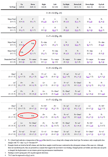
[4.2.5] $\delta^*$ is a convenient shorthand because it lets us focus on chord changes without necessarily having to know the precise starting coordinates within that harmony in the configuration space. Example 37 lists $\delta^*$ for all of the configuration spaces discussed in this article, aside from 3→5→12.
[4.2.6] Due to the persistence of chords across multiple keys in 7→12, $\delta^*$ sometimes lacks the necessary precision to guarantee a specific result, and in those cases it is improper to use it as a shorthand. This occurs four times in Example 37:
- In 3→7→12, moving up from a minor triad may result in $L$ or $T_9$ + dim, depending on the key
- In 3→7→12, moving down from a major triad may result in $L$ or $T_4$ + dim, depending on the key
- In 4→7→12, moving up from m7 may result in $L_2*$ or $T_3$ + M7, depending on the key
- In 4→7→12, moving down from m7 may result in $L_1*$ or $T_8$ + M7, depending on the key
Other times, because of the sometimes unevenly spaced corners, doing $\delta^*(1,1)$ followed by $\delta^*(-1, -1)$ is not an involution. Example 37 is meant to show how broadly applicable $\delta^*$ can be in these configuration spaces; the subsequent notes are meant to show how it is not an operation, but a shorthand that refers to all possible changes from a chord $\mathcal{K}$ given any of the possible coordinates of $\mathcal{K}$.
Context in transformations
[4.3.1] In Tonality and Transformation, Steven Rings (2011) deeply explores some of the implications of scale degree qualia. His ideas resonate with the material in this paper, in the sense that we are not just exploring chords as collections of pcs, but chords as sets contextualized and made distinct by a scale. In Examples 38 and 39 below, evenness-preserving parsimonious transformations are shown in octatonic and diatonic scalar contexts. On the right side of each example are the possibilities for $\delta^*(0,1)$, on the left side of each example are the possibilies for $\delta^*(1, 0)$, and below each example are the possibilities for $\delta^*(1, \pm1)$. On the right side of the diatonic example (Example 39), the neo-Riemannian $L$ transformation is given as a $\delta$ transformation, not $\delta^*$, in accordance with the limitations of the shorthand notation provided above and listed in Example 37.
Example 38. Evenness-preserving neo-Riemannian parsimonious transformations considered in an octatonic scalar context
(click to enlarge) | Example 39. Evenness-preserving parsimonious transformations considered in a diatonic scalar context. P, L, and R are colored to match the coloring in Figure 38
(click to enlarge) |
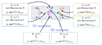
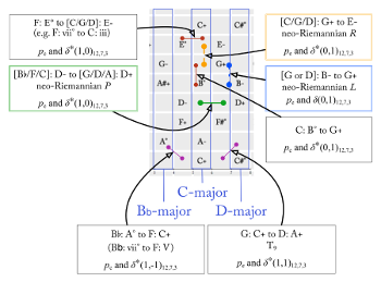
[4.3.2] It is interesting to note the distinctive causes of the neo-Riemannian transformations. For instance, while $R$ is an intra-collection transformation in both the octatonic and diatonic (or, more precisely, can be an intra-collection transformation in the diatonic), $L$ and $P$ result from opposite circumstances. In the diatonic, $L$ is intra-collection and $P$ results from an inter-collection signature transformation $s$ (in the manner of Hook 2008). In the octatonic, $P$ is intra-collection and $L$ results from an inter-collection transformation.(14)
[4.3.3] It is also interesting to consider the role evenness plays in distinguishing parsimonious transformations. All of the chords in a configuration space, rendered through a specific $J$ function, are maximally even and as even as anything else in the same configuration space. The previous discussion noted that a parsimonious transformation G+→B° appears in a 3→7→12 configuration space because it is evenness-preserving, but not in a 3→8→12 configuration space, because the diminished triad is not maximally even in the octatonic. We should also observe that in a pentatonic collection, a diminished triad is not even possible, and in the chromatic we would instead identify as parsimonious any of the 6 trichords caused by a semitone toggle of a pc in G+.
Example 40. φ3/5-space from Yust 2015b

(click to enlarge)
[4.3.4] It seems a good moment to mention the recent work of Jason Yust (2015b), since he has created a chromatic space that is based on the evenness of pc distributions. Yust describes the construction of the neo-Riemannian Tonnetz in “Fourier phase space” (specifically, $\varphi_{3/5}$-space; see Example 40). To understand what that means, let me offer an incredibly brief explanation of DFT phases. The DFT will treat a pitch-class representation of a set as a waveform with peaks and valleys, and a non-multisest representation of each waveform is a series of binary numbers representing the quantity of each pitch class: $\langle pc_0, pc_1, pc_2, pc_3, pc_4, pc_5, pc_6, pc_7, pc_8, pc_9, pc_{10}, pc_{11} \rangle$. The C+ triad would have 1s for $pc_0, pc_4,$ and $pc_7$: $\langle 1, 0, 0, 0, 1, 0, 0, 1, 0, 0, 0, 0 \rangle$. As a waveform, this looks like a square wave with flat-topped mountains at $pc_0, pc_4,$ and $pc_7$, and when that is presented as an input to the DFT, it is decomposed into 12 non-square waveforms that, when added together, would reconstruct the square-wave-style signal of the triad. Each of those partial waveforms is a component of the DFT, $\varphi_n$. A special property of these waveforms is that they are even sinusoids: over the span of an octave (the full possible span of pcs, as octave-equivalent pitches), the second component will have two evenly-spaced peaks, the third component will have three evenly-spaced peaks, etc. Additionally, there is symmetry in the decomposition such that we need only be concerned with the first six components. The more closely a component waveform matches the distribution of pitches in the set, the more relevant that component is to the reconstruction of the square wave, and that relevance is measured in the component’s magnitude. The pcset $\{0, 4, 8\}$ would be well-represented by $\varphi_{3}$, since both are totally even divisions of 12 units into three parts. Because the set class of major and minor triads has ic3, ic4, and ic5, the magnitudes of $\varphi_{3}$ (ic4), $\varphi_{4}$ (ic3), and $\varphi_{5}$ (ic5) are much stronger than the magnitudes of $\varphi_{1}$ (ic1), $\varphi_{2}$ (ic6), and $\varphi_{6}$ (ic2) for a sc(037) triad.
[4.3.5] As one might expect, the magnitudes of the different components of the DFT are identical for any set that is a member of the same set class. Within a set class, what distinguishes one set from another is the phase of each component of the DFT. Put simply, the phase is the amount each component must be offset to match the given pitch-classes. As an example, since G+ is $T_7$(C+), the phases of each component for a G+ triad would in some way come to represent $T_7$ when compared with the phases for the decomposed C+ triad. A Fourier phase space plotting $\varphi_{3}$ against $\varphi_{5}$ emphasizes a relationship between ic4 and ic5, and gives a space that is similar to 3→8→12 configuration space (and therefore also similar to the neo-Riemannian Tonnetz). Its similarity to the configuration space is related to the properties of evenness emphasized in the DFT, but it is dissimilar in that phase space has neither intervals nor harmonies as its core building blocks. Rather, one might separately take a DFT of the pitch C, the pitch E, and the pitch G, and then choose to draw a triangle connecting those pitches in phase space. At the center—and only the center—of that triangle would be the phase of a C+ triad. Movement within that triangle towards the {C, E} dyad could be seen as increasing the volume or quantity (i.e. doublings) of those pitches in the triad, until such a moment that the G is no longer present. Similarly, that {C, E} dyad is only representative of a major third at its center; any inclination towards C or E results in a non-representative version of ic4.(15)
[4.3.6] As compelling as phase spaces are for considering many pcset relationships, phase spaces ultimately represent relationships in chromatic space, and it is the special near-even properties of triads in the chromatic universe that give them a prevalent placement in this space. One can take a 7-component DFT of mod 7 triads to examine the relative evenness of chords within some representative diatonic key, but I’m not aware of a method to represent iterated layers of evenness via this transformation. In this respect, configuration spaces and FiPS are distinctive in their ability to represent harmonic relationships of equally-even chords in a particular scalar context, and their ability to situate G+→B° as appropriately proximal in 3→7→12. Further, it is this representation using FiPS that gives us the ability to find correspondence between cyclic patterns in different spaces, which is the topic of the next section.
Uniform Cycles and Chains of Displacements
[4.4.1] Every maximally even configuration space we have looked at (3→5→12, 3→7→12, 3→8→12, 4→7→12, and 4→9→12) consists of some governing scalar collection and some chordal subset of that collection. The similarity in the construction of the spaces is analytically useful, especially since it allows us to draw strong connections between harmonically dissimilar environments. To uncover some of these connections, I want to focus here on uniform chord cycles.
[4.4.2] Uniform chord cycles consist of a regularly repeating set of displacements at a uniform rate of change. A subset of all possible cycles can be clearly expressed in a configuration space by drawing a completely straight line between any two identical harmonies.(16) Yust 2013a identifies this type of cycle as having second-order uniformity, and as being “highly non-trivial” with respect to analytical applications. In contrast to a cycle that might involve regularly repeating transformations at a non-uniform rate of change, a uniform cycle may consistently be characterized by a line with a slope $\mathbb{M}$, and often as a short series of $\delta$ or $\delta^*$ operations repeated a specific number of times.(17)
[4.4.3] The previously-shown uniform cycles can be characterized using $\delta^*$ as follows:
- Example 29 (A $PR$ cycle in a 3→7→12 configuration space) shows the a cycle $\langle \delta^*(1,0), \delta^*(0,1) \rangle^4_{12,7,3}$ starting at a C− triad.
- Example 30 (A $PL$ cycle in a 3→7→12 configuration space) shows $\langle \delta^*(1,0), \delta^*(1,-1) \rangle^3_{12,7,3}$ starting at a D− triad.
- Example 31 (An $LR$ cycle in a 3→7→12 configuration space) shows a portion of $\langle \delta^*(0,-1), \delta^*(1,-1) \rangle^{12}_{12,7,3}$ starting at a G− triad.
- Example 32 (An $LR$ cycle in a 3→5→12 configuration space) shows $\langle \delta^*(1,0), \delta^*(0,1) \rangle^{12}_{12,5,3}$ starting at a C− triad.
- Example 34 (A <$P_1*, P_2*, R*$> cycle in a 4→7→12 configuration space) shows $\langle \delta^*(1,0), \delta^*(0,1), \delta^*(1,0) \rangle^3_{12,7,4}$ starting on C#m7.
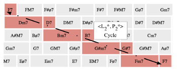
- Example 35 (An <$L_2*, P_2*$> cycle in a 4→7→12 configuration space) shows $\langle \delta^*(1,-1), \delta^*(1,0) \rangle^4_{12,7,4}$ starting on F7.
[4.4.4] Unlike the six other uniform cycles listed above, Example 36 (a cycle in a 4→7→12 configuration space that augments an <$L_1*, L_2*, R*$> cycle) cannot be characterized using $\delta^*$, because of its movement into and out of m7 chords (excluded from $d^*$ according to Example 37). In this scenario, to properly express $\delta$ we must determine the repeated harmonic pattern as well as the slope of the line from that pattern. There is a four-chord pattern that repeats six times, adjusted each time by $T_2$, before the uniform cycle completes. The slope of a line drawn from the top left corner of a half-diminished chord to the top left corner of the next half-diminished chord ($T_2$ of the first) is $\mathbb{M} = - \tfrac{3}{2}$, which can be understood as a line that travels three units down and two units to the right. This relates $m_1$ to $m_2$ as $m_2 = - \tfrac{3}{2} m_1$, and those values will always appear in that relationship in any $\delta$ operation. Because a four-chord pattern is repeated six times over the course of the cycle, we want four $\delta$ operations in series. Assuming a start at the top-left corner of a half-diminished seventh chord, the chain of displacements will be $\langle \delta(\tfrac{2}{3}, -1), \delta(\tfrac{1}{3}, -\tfrac{1}{2}), \delta(\tfrac{1}{3}, -\tfrac{1}{2}), \delta(\tfrac{2}{3}, -1) \rangle^6_{12,7,4}$. It is also worth noting that we now have the language to address the inability of Example 36 to represent an <$L_1*, L_2*, R*$> cycle with a straight line: in a 4→7→12 configuration, that cycle is non-uniform. One way to characterize the cycle might be $\langle \delta(\tfrac{1}{3}, -1), \delta(\tfrac{2}{3}, -1), \delta(1, -1) \rangle^6_{12,7,4}$, and this non-uniform characterization has no equation that can relate $m_1$ to $m_2$.
Example 41. Parsimonious cycles with negative slope in a 3→8→12 configuration space
(click to enlarge)
[4.4.5] Example 23 labels straight lines indicating $PR$, $LR$, and $LP$ cycles in a 3→8→12 configuration space. Example 41 represents all possible $LP$ cycles in the 3→8→12 configuration space. Each cycle in Example 41 is represented by a line with the same slope $\mathbb{M} = -\frac{1}{4}$. In this case, the slope tells us that the governing scale collection (adjusted by changes to $m_1$) changes sharp-wise at a rate 4x faster than the root-lowering intra-scale transformations represented by changes to $m_2$. In addition to the shared slope between cycles, each cycle is distinguished by a constant $b$ that alters the chord on which the cycle starts. The cycle with D+ has $b=5.5$ ($m_2 = -\frac{1}{4}m_1+5.5$), the cycle with F+ has $b=3.5$, and the cycle with E+ has $b=1.5$. These constants indicate the $m_2$ value when $m_1=0$.
Example 42. Un-parsimonious cycles with negative slope in a 3→8→12 configuration space
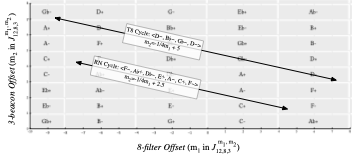
(click to enlarge)
[4.4.6] There are some related uniform cycles in this configuration space, as shown in Example 42. What is distinctive about these cycles is that, despite the shared slope of the line from Example 41, neither consists of wholly parsimonious changes between the triads. In the case of the cycle <F−,
[4.4.7] In all scalar configuration spaces, including the neo-Riemannian-Tonnetz-isomorphic 3→8→12 space, there will consistently be chord-to-chord boundaries that are un-parsimonious. If we are concerned entirely with parsimonious chord changes, then we may choose to ignore patterns and transformations that intersect these boundaries; if we instead choose to look at the wider grouping of cycles caused by uniform rates of change and repeated displacement operations, then we may include patterns such as those in Example 42. The difference between an $NR$ cycle and an $LP$ cycle in this space is nothing more than the specifics of the chord boundary; both cycles may be described as $\langle(d^*(1,0), d^*(0,1))\rangle^3$, and it is only the starting chord that differs. (The $T_8$-cycle is a special case in which only corner boundaries are crossed, $\langle(d^*(1,1)\rangle^3$, though one can still see $d^*(1,1)$ as an explicit simultaneity of $d^*(1,0)$ and $d^*(0,1)$.)
Example 43. Indicators of un-parsimonious boundaries in a 3→8→12 configuration space
(click to enlarge)
[4.4.8] With respect to visualizing parsimonious and un-parsimonious displacements, Example 43 indicates un-parsimonious boundaries with a red mark. As shown in Example 37, all transformations between two adjacent corners will be un-parsimonious, as in the T8 cycle, and every other chord pair affected by scalar transformation will not be parsimonious, as in the $RN$ cycle. The un-parsimoniousness at the corners results from simultaneous changes within and between scales; the un-parsimoniousness at alternating edges results from the non-coprime relationship of 8 and 12.
Example 44. Cycles with negative slope in a 3→7→12 configuration space
Y is T4(X), Z is T4(Y), X is T4(Z)
X# is T1(X), Y# is T1(Y), Z# is T1(Z)
Y is T3(X#), Z is T3(Y#), X is T3(Z#)
(click to enlarge)
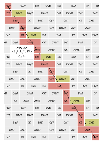
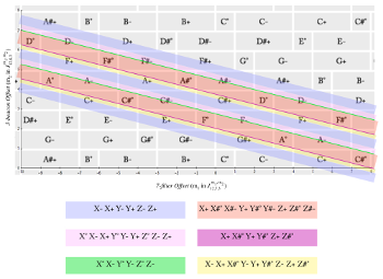
[4.4.9] The diatonic trichord space (3→7→12) has a much broader array of cycles than the octatonic trichord space, due to the irregular sizing and distribution of chords in the configuration space. No edges are un-parsimonious, because 3 is coprime with 7 and 7 is coprime with 12; un-parsimonious transformations occur consistently and exclusively at adjacent corners (Example 37 can serve as a reference for the relationships at these boundaries). Continuing to focus on the $LP$ cycle, Example 44 identifies the $LP$ cycle in this diatonic trichord space, along with all other uniform cycles that have the same rate of change (transpositions of $m_2 = -\frac{1}{4}m_1$). Six bands of color are used to indicate the regions in which the cycles occur. Example 44 also provides a color-coded key to the overall harmonic patterns. Of these patterns, three are enneatonic, three are hexatonic (including $LP$), and two of the hexatonic cycles are un-parsimonious. These two un-parsimonious hexatonic cycles, indicated in green and fuschia, are special in that the regions have zero area, and in both cases include corner boundary $d^*(1, -1)$ displacements.
Example 45. Plot of diatonic cycles defined by a slope of 𝕄 = −¼ in a 3→7→12 configuration space
(click to enlarge)
[4.4.10] The cycles in Example 44 follow a consistent (though incomplete) pattern of permutations that divide the octave into three major-third-related groups. Let’s take the pink cycle, <X° X− X+ Y° Y− Y+ Z° Z− Z+>, as the most representative cycle. The main distinction between the pink pattern and the standard hexatonic LP cycle is that the latter traverses the configuration space in a way that avoids the diminished chord. A different permutation on chord-avoidance shows up along the green line. In this pattern, the major chord is omitted instead of the diminished chord. We do not see the minor-chord-omitting pattern <X° X+ Y° Y+ Z° Z+> in Example 44, because that particular cycle occurs when the slope is $\mathbb{M} = +\frac{1}{3}$ (instead of the $\mathbb{M} = -\frac{1}{4}$ under examination here).(18) Example 45 attempts to classify these diatonic cycles with some manner of conventional naming.
Beyond a basic configuration space
[5.1.1] In a FiPS configuration of 7→12 with an initial offset of $m_1=0$, we get a
Example 46. Ordered output of C Ionian and D Dorian, at $ J^{5}_{12,7}$ and $ J^{17}_{12,7}$, respectively.
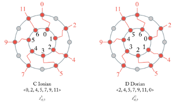
(click to enlarge)
[5.1.2] One consequence of treating the output of FiPS as a family of ordered sets is that the configuration spaces reflect a more concrete measure of voice-leading distance. For instance, in an ordered 3→7→12 configuration space, C+ $\xrightarrow{\delta^*(0, 1)_{12,7,3}}$ A− will be one of $\langle 0, 4, 7\rangle \rightarrow \langle 0, 4, 9\rangle$, $\langle 4, 7, 0\rangle \rightarrow \langle 4, 9, 0\rangle$, or $\langle 7, 0, 4 \rangle \rightarrow \langle 9, 0, 4\rangle$, depending on the exact rotational offset of the 7-hole filter. And in an ordered 7→12 configuration space in which one wants to consider modes (Example 46), C Ionian is more proximal to G Ionian ($\delta^*(1)_{12,7}$) than it is to D Dorian ($\delta^*(1)^{12}_{12,7}$)—take note of the exponentiation in the latter equation.
[5.1.3] When looking at chords and scales as ordered pcsets, there seem to be common and intuitive ways of discussing sets consisting of identical pcs. With seventh chords, we usually refer to root position, first inversion, second inversion, and third inversion as a means of identifying the first and lowest pitch in the presentation of that chord. The ordinals are not random; if the pitch classes are ordered in their most compact form starting from the chord root, it is the first, then second, then third, then fourth note that takes its place on the bottom. With modes, we have a similar manner of discussion: the mode after Ionian is Dorian, and the mode after Dorian is Phrygian. The ordering of those modes is based on the stepwise shift of the final.
[5.1.4] There is something reminiscent of parsimony in these orderings, in the sense that neighboring inversions and neighboring modes represent the most frugal changes to a set or collection’s order. With FiPS (and the $J$ function), these incremental changes of order are arranged by placing two filters of identical cardinality in series. Let’s try this first with a configuration of 3→3→7→12, which, to distinguish the 3-hole beacon and filter, could be written as 3(inner)→3(outer)→7→12. The 3(outer)→7→12 filters will operate in the now-familiar diatonic triad configuration space. The inner 3-hole beacon does not alter the pitch classes in the sets; rather, it alters the inversions of the triads by frugally shifting the order of the pcs. Above, $\langle 0, 4, 7\rangle \rightarrow \langle 0, 4, 9\rangle$ was given as one possible version of C+ $\xrightarrow{\delta^*(0, 1)_{12,7,3}}$ A−, and it is also a version of C+ $\xrightarrow{\delta^*(0, 1, 0)_{12,7,3,3}}$ A−. But where $\langle 0, 4, 7\rangle$ and $\langle 4, 9, 0\rangle$ cannot be adjacent in an ordered two-dimensional configuration space of 3→7→12, the ordered three-dimensional configuration space of 3→3→7→12 makes that possible with $\langle 0, 4, 7\rangle \xrightarrow{\delta^*(0, 1, 1)_{12,7,3,3}} \langle 4, 9, 0\rangle$. Although the transformation from C+ to A− is conventionally parsimonious, and although the inversion of a chord on its own is a frugal change, the combination of both changes here shows a more disjunct change in voice-leading—the type of disjunction that is typical of corner-boundary traversal in a configuration space.
[5.1.5] Of note in these discussions of ordering is that, until one introduces a rotational transform using 3→3, no crossing voice leadings are possible, which relates to the voice-leading spaces discussed by Tymozcko (2011), Yust (2015b and Hall (2009).(19) What is unique about FiPS is that it allows us to treat that condition as either one that must be overcome through a great leap in the space, or—using a configuration in which rotations are allowed—allows us to more conventionally represent a voice crossing as a boundary condition across a different axis of movement. We may choose to remain in an ordered two-dimensional space in which it takes a large translation to get from $\langle 0, 4, 7\rangle$ to $\langle 4, 9, 0\rangle$, or we can represent that translation in a different dimension using a 3(inner)-beacon.(20) In this sense, nested rings of the same cardinality are not a trick of FiPS in which particular relationships are achieved; rather, nested rings of the same cardinality move what would be a large voice-leading traversal in one dimension into a short traversal in a different dimension. I think the latter representation can be particularly effective for analysis.
[5.1.6] An interesting configuration space—one which I find analytically useful—is a three-dimensional space generated by 3→7(inner)→7(outer)→12. As it was with the 3→3→7→12 configuration, this space operates generally within the diatonic trichord space, here represented by 3→7(outer)→12. The 7(inner) filter causes a frugal displacement of scale degrees, in the same manner one might assign the first scale degree to the consistently shifting finals in the list of modes discussed above. In this way, a triad altered by a shift in the 7(inner) filter could be expressed with scale degrees as $\langle \hat{0}, \hat{2}, \hat{4} \rangle \xrightarrow{\delta^*(0, 1, 0)_{12,7,7,3}} \langle \hat{1}, \hat{3}, \hat{5} \rangle$, or without regard to ordering as C+→D−. This is as unparsimonious a transformation as possible between triads in a diatonic collection, yet the displacement of scale degrees is as frugal as possible. As we have previously seen, what is parsimonious or frugal in an isolated configuration, such as shifts between octatonic collections, does not necessarily yield parsimonious or frugal results.
[5.1.7] A key-of-C-major slice of the three-dimensional configuration space generated by 3→7(inner)→7(outer)→12 is given in Example 47. Example 48 shows all possible $\delta^*$ relationships from a C+ triad in all three dimensions of the configuration space. With respect to Example 47, the changes brought about by the 3-hole beacon are all parsimonious; the changes brought about by the 7(inner)-filter are all unparsimonious, and could be expressed by the scalar transposition $t_1$. I find it interesting that the dominant and subdominant in this space sit at opposing corners, making them higher-order transformations in terms of $\delta^*$, and uniquely higher-order (as opposed to the other chords at corner boundaries that also appear at non-corner boundaries). This configuration resembles Lerdahl’s model from Tonal Pitch Space (2001), but the resemblance is not something that supports or suggests similar reasoning to Lerdahl. Rather, the configuration space presented here results from bringing into its own dimension the alteration of chord roots by $t_1$ (in lieu of having large vectors between chords in an ordered 3→7→12 configuration space).
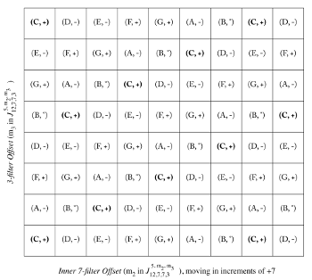
Example 47. The configuration space of the 3-beacon and inner 7-filter in a 3→7(inner)→7(outer)→12 FiPS configuration, expressed in the key of C-major with m1 = 5
(click to enlarge) | Example 48. A three-dimensional plot of 3→7(inner)→7(outer)→12 configuration space, where each vertical layer represents key changes caused by the outer 7-filter. Relationships relative to a C+ tonic chord are shown
(click to enlarge) |
Example 49. A 3→7→7→12 FiPS configuration in which the inner 7-filter moves each C-major-constrained harmony up by t1
(click to watch video)
[5.1.8] Example 49 provides an animation of the FiPS rings, in which only the inner 7-filter rotates. The series of chords shown in the example is C+→D−→E−→F+→G+→A−→B°→C+, an ascending series of $t_1$ transpositions in the key of C major.
Analysis with order-shifted sets
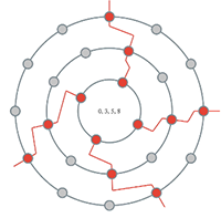
[5.2.1] Compared to the configuration spaces of the previous sections, I think it is less clear what impact higher-order iterated maximally-even sets might have on analysis. I will show here a speculative analysis of the third phrase of Chopin’s Op. 28, No. 9 Prelude in E major. This analysis takes place in a 3→7(inner)→7(outer)→12(inner)→12(outer) FiPS configuration, though our focus will not be on the role of the inner 12-filter (which displaces the pcs by chromatic step, as shown in Example 50). Rather, this analysis focuses on the role of the intra-key actions of the 3-beacon and inner 7-filter. Example 51 is the excerpt of the Prelude under consideration. Example 52 is a lengthy representation of every harmony in the figure as the product of a $J$ function, and the $\delta$ operation (or $\delta^*$ representation of $\delta$) that transforms each chord to the next. Example 53 is a detailed animation of the entire phrase expressed in a FiPS configuration of 3→7→7→12→12. If you scan through the $\delta^*$ values for $m_3$ and $m_4$ in Example 52, or scrub through Example 53 quite slowly, you will see repetitive patterns in the 3-beacon and inner-7-filter. To make this more visible, Example 54 shows the motion of only the 3-beacon (with the inner 7-filter stabilized), and Example 55 shows the motion of the 3-beacon and the inner 7-filter, with the outer 7-filter stabilized.
Example 50. A 3→7→7→12 FiPS configuration in which the inner 12-filter moves each harmony up by T1
(click to watch video) | Example 51. The final phrase of Chopin’s Op. 28, No. 9 Prelude in E major, mm. 9–12
(click to enlarge) |
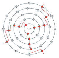
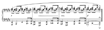
Example 52. J representations of every chord in the final phrase of Chopin’s prelude, paired with the δ* representations of the operations that incrementally change the output of FiPS
(click to enlarge and see the rest) | Example 53. The final phrase of Chopin’s prelude, represented by a 3→7→7→12 FiPS configuration
(click to watch video) |
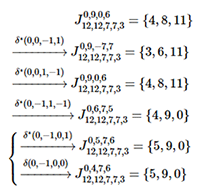
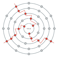
Example 54. The material from Example 53, isolating the rotations of the 3-beacon
(click to watch video) | Example 55. The material from Example 53, isolating the rotations of the 3-beacon and inner 7-filter
(click to watch video) |
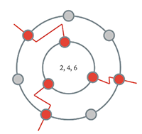
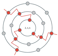
Example 56. A plot of the rotational offsets of the 3-beacon and inner 7-filter from Example 53
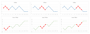
(click to enlarge)
[5.2.2] The pair of motions from the 3-beacon and inner 7-filter is precisely repeated three full times, once for each group of four chords. Example 56 graphs the rotational offsets of the 3-beacon in the top trio of graphs, and the rotational offsets of the inner 7-filter in the bottom trio of graphs. Each repetition of the four-chord pattern is highlighted in red. The music has a sequential sound: it moves from E major to F major, then suggestively to G major, and finally returns to E major. But, as we begin to explore the sequence in the music, it does not conform to the rigidity of pattern suggested by the motions of the 3-beacon and inner 7-filter.
[5.2.3] The four-chord groups are not truly sequential. The first three chords belong to E major (E: I V I), and the fourth chord is an A− triad. A− is a chord achieved through mixture, meaning that we conceive of it as a chord belonging to E minor. The $\delta^*(0, -1, 0, 1)$ operation on the second E+ harmony moves $m_2$ from 9 to 6, which is, in FiPS, a representation of G major / E minor. The key shifts again as the sequence starts in F major, making the borrowed E: iv chord a pivot to F: iii. Unlike the previous four-chord group, this group stays in its key (F: I V I IV), with no alterations to the fourth chord. But instead of shifting to G major at the start of the third four-chord group, a G− triad appears, which is diatonic to the previous F major group. Musically, we might make arguments that the sequence starts in minor, not major, but it is also worth noting that the F major membership of the G− triad brings with it some ambiguity. By means of $\delta(0,-1,0,0)^2$ on the G minor triad $\{7, T, 2\}$, G− changes from Dm: iv to Cm: v, and does not stabilize as a local tonic before other chromatic shifts lead to G: V I. The tonicization of G+ is followed by a rather dramatic chromatic shift to E major.
[5.2.4] As explained in the previous paragraph, the 4-chord pattern in the music—E: I V I x, F: I V I x, G: i V I x—is not entirely consistent, and I would argue that part of the intrigue of this passage is that we can simultaneously hear it as both a regular pattern and an irregular one. FiPS is showing absolute consistency at the intra-key level, and this may offer some guidance as to why are able to hear a sequence: there is a consistent diatonic pattern that runs as an undercurrent to the less consistent key areas and modal borrowings.
Final Thoughts
[5.3.1] In this paper I started by examining maximally even sets, Filtered Point-Symmetry, and the $J$ function. I then explored configuration spaces and scalar contexts as useful theoretical models that can be understood in terms of multiple layers of evenness working in concert. Among other things, configuration spaces allow us to examine and compare harmonic relationships in different scales, such that an L transformation is not the same in a diatonic configuration as it is in an octatonic configuration, even when the pcs are the same. I pursued the concept of distinctive, scale-based harmonic relationships more deeply by examining the historical use of parsimony, and by presenting a displacement operation that helps to codify the traversal of a configuration space. I also looked at uniform cycles in different configuration spaces. Finally, I examined multi-dimensional configuration spaces as a means of moving crossing voice leadings into a different dimension, and as a potential means of analyzing music. I hope the reader agrees that FiPS and its configuration spaces are able to deliver many interesting and analytically fruitful insights into harmonic relationships.
Richard Plotkin
University at Buffalo
richardjplotkin@gmail.com
Works Cited
Callender, Clifton. 1998. “Voice-leading Parsimony in the Music of Alexander Scriabin.” Journal of Music Theory 42 (2): 219–33.
Callender, Clifton, Ian Quinn, and Dmitri Tymoczko. 2008. “Generalized Voice-Leading Spaces.” Science 320 (5874): 346–48.
Childs, Adrian P. 1998. “Moving Beyond Neo-Riemannian Triads: Exploring a Transformational Model for Seventh Chords.” Journal of Music Theory 42 (2): 181–93.
Clough, John, John Cuciurean, and Jack Douthett. 1997. “Hyperscales and the Generalized Tetrachord.” Journal of Music Theory 41 (1): 67–100.
Clough, John, and Jack Douthett. 1991. “Maximally Even Sets.” Journal of Music Theory 35 (1/2): 93–173.
Clough, John, Nora Engebretsen, and Jonathan Kochavi. 1999. “Scales, Sets, and Interval Cycles: a Taxonomy.” Music Theory Spectrum 21 (1): 74–104.
Cohn, Richard. 1996. “Maximally Smooth Cycles, Hexatonic Systems, and the Analysis of Late-Romantic Triadic Progressions.” Music Analysis 15 (1): 9–40.
—————. 1997. “Neo-Riemannian Operations, Parsimonious Trichords, and Their ‘Tonnetz’ Representations.” Journal of Music Theory 41 (1): 1–66.
—————. 2000. “Weitzmann’s Regions, My Cycles, and Douthett's Dancing Cubes.” Music Theory Spectrum 22 (1): 89–103.
—————. 2003. “A Tetrahedral Model of Tetrachordal Voice Leading Space,” Music Theory Online 9/4.
—————. 2012. Audacious Euphony: Chromaticism and the Consonant Triad’s Second Nature. Oxford University Press.
Douthett, Jack. 2008. “Filtered Point-symmetry and Dynamical Voice-leading.” In Music Theory and Mathematics: Chords, Collections, and Transformations, edited by Jack Douthett, Martha M. Hyde, and Charles J. Smith, 72–106. University of Rochester Press.
Douthett, Jack, and Peter Steinbach. 1998. “Parsimonious Graphs: A Study in Parsimony, Contextual Transformations, and Modes of Limited Transposition.” Journal of Music Theory 42 (2): 241–63.
Hall, Rachel Wells. 2009. “Linear Contextual Transformations.” In Quaderni di Matematica: Theory and Applications of Proximity, Nearness and Uniformity, edited by Somashekhar Naimpally and Giuseppe Di Maio, 101–30. Dipartimento di Matematica della Seconda Università degli Studi di Napoli.
Hook, Julian. 2008. “Signature Transformations.” In Music Theory and Mathematics: Chords, Collections, and Transformations, edited by Jack Douthett, Martha M. Hyde, and Charles J. Smith, 137–60. University of Rochester Press.
Lerdahl, Fred. 2001. Tonal Pitch Space. Oxford University Press.
Lewin, David. 1987. “Some Instances of Parallel Voice-Leading in Debussy.” 19th-Century Music 11 (1): 59–72.
—————. 2001. “Special cases of the interval function between pitch-class sets X and Y.” Journal of Music Theory 45 (1): 1–29.
Plotkin, Richard. 2010. “Transforming Transformational Analysis: Applications of Filtered Point-Symmetry.” Ph.D. diss., University of Chicago.
—————. 2011. “Cardinality Transformations in Diatonic Space.” Mathematics and Computation in Music MCM 2011, 207–19. Lecture Notes in Computer Science, vol 6726. Springer.
Plotkin, Richard and Jack Douthett. 2013a. “Scalar Context in Musical Models.” Journal of Mathematics and Music 7 (2): 103–25.
—————. 2013b. “Thoughts and Reactions.” Journal of Mathematics and Music 7 (2): 167-173.
Quinn, Ian. 2006. “General Equal-tempered Harmony (Introduction and Part I). Perspectives of New Music 44 (2): 114–58.
—————. 2007. “General Equal-tempered Harmony, II and III.” Perspectives of New Music. 45 (1): 4–63.
Rings, Steven. 2011. Tonality and Transformation. Oxford University Press.
Straus, Joseph. 2005. “Voice Leading in Set-Class Space.” Journal of Music Theory, 49 (1): 45–108.
Tymoczko, Dmitri. 2008. “Scale Theory, Serial Theory and Voice Leading.” Music Analysis 27 (1): 1–49.
—————. 2011. A Geometry of Music: Harmony and Counterpoint in the Extended Common Practice. Oxford University Press.
Yust, Jason. 2013a. “Tonal Prisms: Iterated Quantization in Chromatic Tonality and Ravel's ‘Ondine.’” Journal of Mathematics and Music 7 (2): 145–65.
—————. 2013b. “A Space for Inflections: Following Up on JMM’s Special Issue on Mathematical Theories of Voice Leading.” Journal of Mathematics and Music 7 (3): 175–93.
—————. 2015a. “Voice-Leading Transformation and Generative Theories of Tonal Structure.” Music Theory Online 21/4.
—————. 2015b. “Schubert’s Harmonic Language and Fourier Phase Space.” Journal of Music Theory 59 (1): 121–81.
Footnotes
1. The seasoned scale theorists to whom I refer would be familiar with Clouth and Douthett 1991; Clough 1999; Douthett 2008; and Plotkin and Douthett 2013a and 2013b.
Return to text
2. I use diatonic to refer exclusively to set class [7-35]. I use heptatonic to refer more generically to a 7-note collection.
Return to text
3. A more familiar simple quantization function is rounding, which takes any fraction to its nearest integer, instead of the lowest integer.
Return to text
4. A discussion of harmonies preserving “as many common tones as possible” begins to encroach on concepts of voice-leading parsimony. This connection is further explored in the “Parsimony and Displacement” section below.
Return to text
5. Plotkin and Douthett 2013a goes into greater detail on these isomorphisms.
Return to text
6. A detailed discussion of parsimony appears in 4.1.1–4.1.7. Although this cycle of diatonic trichords is not a neo-Riemannian cycle of chords belong to sc(037), it is indeed parsimonious.
Return to text
7. When I refer to inconsistent usages of the term “voice-leading parsimony,” I am thinking of the aggregate of Cohn 1996, 1997, 2000, 2003; Callender 1998; Douthett and Steinbach 1998; Childs 1998; Straus 2005; and Tymoczko 2008.
Return to text
8. A nice example of the lack of consensus around interval limits is in Callender 1998: “Another consideration in the formalization of parsimonious voice leading is the intervallic limitation of moving voices. Cohn limits motion of voices to no more than a whole-step, Childs to a half-step, and Douthett and Steinbach keep track of half- and whole-steps separately. Since the interval vector for set class 6-34 contains a high proportion of whole-steps, I shall limit conjunct voice leading to the half-step” (221–22).
Return to text
9. By “similarly even,” I mean to refer to a limited family of set classes that have similar (and high) evenness—for example, a family of set classes that includes augmented triads (totally even) along with major and minor triads.
Return to text
10. CQT voice-leading spaces model both evenness relationships and voice-leading relationships between all sets (or set classes, depending on OPTIC equivalence). This is notably distinct from other approaches to parsimony that focus on chords that are nearly-even or an abundance of set classes.
Return to text
11. It is possible that such an approach could lead to a more specific characterization of un-parsimoniousness, where a 3-note change in a 3-note triad is more un-parsimonious than a 2-note change in a 3-note triad. In this paper, I have kept the simpler characterization, where something is or is not parsimonious.
Return to text
12. Such a perspective strongly evokes scale degree qualia as proposed by Steve Rings in Tonality and Transformation (2011), further discussed in 4.3.1.
Return to text
13. Douthett 2008 proposed stroboscopic portraits as a means of examining non-consecutive pc set output in FiPS. Treating each \(m_n\) as a function of time \(m_n(t)\), a stroboscopic portrait captures the output of the system at specific intervals of \(t\). If, for instance, the output of a configuration were <C+, A-, A+,
Return to text
14. These properties are discussed to some extent in Plotkin and Douthett 2013a and 2013b.
Return to text
15. A short yet thorough synopsis of the math in Yust's article is summarized at http://www.eamonnbell.com/blog/2017/04/22/introducing-the-dft/.
Return to text
16. In fact, the straight line must also intersect the same portion of the harmony, as shown in the subsequent examples.
Return to text
17. Slope is usually represented by \(m\), but I have chosen \(M\) here to avoid confusion with \(m_n\) from the \(J\) function.
Return to text
18. A table of all possible patterns appears in Plotkin 2011, though the patterns are not as clearly identified by their transpositional and permutational relationships. Some related thoughts appear in Plotkin 2010.
Return to text
19. The lack of crossing voice leadings is important in the work of Tymoczko 2008 and Hall 2009.
Return to text
20. As previously discussed in relation to \(\delta\) operations with values greater than 1, such leaps can be treated in the manner that Douthett 2008 approaches stroboscopic portraits.
Return to text
Copyright Statement
Copyright © 2019 by the Society for Music Theory. All rights reserved.
[1] Copyrights for individual items published in Music Theory Online (MTO) are held by their authors. Items appearing in MTO may be saved and stored in electronic or paper form, and may be shared among individuals for purposes of scholarly research or discussion, but may not be republished in any form, electronic or print, without prior, written permission from the author(s), and advance notification of the editors of MTO.
[2] Any redistributed form of items published in MTO must include the following information in a form appropriate to the medium in which the items are to appear:
This item appeared in Music Theory Online in Volume 25, Issue 2 in July 2019. It was authored by Richard Plotkin (richardjplotkin@gmail.com), with whose written permission it is reprinted here.
[3] Libraries may archive issues of MTO in electronic or paper form for public access so long as each issue is stored in its entirety, and no access fee is charged. Exceptions to these requirements must be approved in writing by the editors of MTO, who will act in accordance with the decisions of the Society for Music Theory.
This document and all portions thereof are protected by U.S. and international copyright laws. Material contained herein may be copied and/or distributed for research purposes only.

Prepared by Michael McClimon, Senior Editorial Assistant
Number of visits:
15916