Some Proposed Enhancements to the Operationalization of Prominence: Commentary on Michèle Duguay’s “Analyzing Vocal Placement in Recorded Virtual Space”
Trevor de Clercq
KEYWORDS: Virtual Space, Voice, Vocal Placement, Popular Music, Rihanna, Eminem
ABSTRACT: This article offers an alternate methodology for quantifying the parameter of prominence introduced by Duguay (2022) to describe the relative level of the voice in the mix. I begin with a discussion of RMS amplitude, focused on the difference between average and true RMS values. I then propose that overall RMS amplitude ratios be logarithmically transformed to more closely represent the perception of relative level differences, with the relative level of the vocal better assessed through comparison to the mix minus the vocal rather than the full mix. I also discuss methods to compensate for the uneven sensitivity of the human ear to different frequencies at different sound pressure levels, ultimately recommending that prominence be quantified in terms of K-weighted loudness units. I conclude with a reconsideration of vocal prominence in the four Rihanna and Eminem collaborations that Duguay analyzes in her original article.
DOI: 10.30535/mto.30.1.2
Copyright © 2024 Society for Music Theory
I. Introduction
[1.1] It is well known that the traditional domains of music theory—e.g., melody, harmony, rhythm, and form—offer only a narrow perspective on the full listening experience of recorded music, perhaps especially modern popular music. If a researcher wants to describe the virtual space of a sound recording, for example, they will likely need to engage with concepts from the field of audio engineering, such as compression, equalization, and reverberation. Yet musicologists rarely have any significant technical training in this area. Consequently, as Michèle Duguay notes in the December 2022 issue of this journal ([2.7–10]), previous analyses by musicologists have lacked any explicit methodology or replicable procedure that would allow different virtual spaces to be consistently compared.
[1.2] In response, Duguay presents an empirical method based on digital sound processing tools that allows a researcher to more precisely locate recorded sound sources in a virtual space. In particular, Duguay focuses on how to analyze the placement of the voice in a mix. Her proposed method defines five parameters for this task: width, pitch range, prominence, environment, and layering. After describing in detail how to calculate these five parameters through a combination of aural analysis and audio feature extraction, Duguay illustrates the value of her approach through a close analysis of vocal placement in four collaborative songs by Eminem and Rihanna.
[1.3] I agree with Duguay that if a researcher wants to study the placement of a sound source within a virtual space, it is useful if not vital to have well-defined ways of measuring the various aspects that characterize that space. If these quantitative tools are to be meaningful, I would also add, they should correspond as closely as possible to our perceptual experience. With these goals in mind, this commentary builds on Duguay’s original formulation of prominence with some thoughts on how the parameter of prominence may be better operationalized.
[1.4] The discussion below is organized into three main sections, each of which offers a successive improvement to how prominence is measured. The first section describes a more accurate method for calculating the overall level of an audio signal in terms of its RMS amplitude, which is the basis of Duguay’s formula for prominence. As I will show, average and true RMS values are not identical, although differences in experimental methods may result in variances larger than the differences between these values. The second section proposes that ratios of these overall RMS values should be logarithmically transformed to more closely represent the perception of relative level differences, which are typically measured in decibels. I also argue that the relative level of the vocal is better assessed through comparison to the mix minus the vocal rather than the full mix. Finally, the third section describes methods to compensate for the uneven sensitivity of the human ear to different frequencies at different sound pressure levels. Ultimately, I recommend that prominence be quantified as loudness units (LU) on a K-weighted LUFS scale.
[1.5] The ensuing discussion requires some technical detail from the field of audio engineering, including some mathematical manipulations (although none higher than high-school level).(1) The good news, as I discuss in section 4 below, is that existing software tools will perform these calculations automatically. My proposal, therefore, not only improves the accuracy and perceptual relevance of prominence values, it also reduces the amount of computation involved, which hopefully ensures more consistent as well as more meaningful measurements between researchers.
2. RMS Amplitude
[2.1] Duguay’s method for calculating vocal prominence first requires that the vocal track of the song be isolated from the original mix as a separate audio file. There are a number of ways to do this, as she explains, one of which is to use the freely available Open-Unmix software (Stöter et al. 2019). With the vocal track isolated as a separate audio file, Duguay defines the prominence of the voice as the ratio of the RMS (“Root-Mean-Square”) amplitude of the vocal track to the RMS amplitude of the mix overall ([3.14]). Specifically, Duguay’s proposed formula for vocal prominence is
where the multiplication by 100 converts the proportion into a percentage.
[2.2] To support this formulation, Duguay explains in footnotes 23 and 24 that the amplitude of an audio signal is related to (although not the same as) the perceived loudness of that signal: generally speaking, greater signal amplitude corresponds to an increase in perceived loudness. Furthermore, the RMS amplitude of an audio signal indicates the amplitude of that signal over some period of time. These RMS amplitude levels, she notes, can be automatically extracted using an add-on coded by Jamie Bullock within the Sonic Visualiser software. Duguay then offers an example of calculating prominence based on the opening vocal hook sung by Rihanna in the Eminem song “Love the Way You Lie” (2010). Plugging in average RMS amplitude values computed elsewhere, Duguay reports for this opening hook that
Given this result, Duguay states that Rihanna’s voice “occupies approximately 85.5% of the chorus’s amplitude” ([3.14]). In other words, the vocal has a relatively high level—and is thus rather prominent—within the overall mix.
[2.3] Duguay’s formula for prominence is a reasonable first step for attempting to assess the relative level of the vocal (or other isolated track) in the mix. But as I show in this section and those that follow, there are some enhancements to this formulation that can make it more accurate, more reliable, more interpretable, and more representative of human perception. I will explain these enhancements in stages, each building on the previous. In this first stage, the improvement will be fairly small, but it will lay the foundation for the more significant enhancements discussed in the sections that follow.
[2.4] To begin, it will be helpful to understand how (and why) to calculate an RMS amplitude. Sound, of course, is caused by vibrations within a medium, which can be represented by oscillations around a central value of zero. In this model, the instantaneous amplitude of a sound wave varies over time between positive values (compressions) and negative values (rarefactions). To calculate the overall amplitude of an audio signal, it would not be useful to take the arithmetic mean of these instantaneous amplitude values, since the positive and negative values would cancel out; the result would be an overall amplitude of zero for typical periodic signals, no matter how loud or quiet.
[2.5] Instead, as Duguay explains, audio engineers measure signal level in terms of its RMS amplitude. The procedure for calculating the RMS amplitude of a signal is as follows: first square each instantaneous amplitude value (to avoid the positive and negative values from canceling out), then take the arithmetic mean of these squared values, and finally take the square root of this mean. (To be clear, the order of steps is not: first take the square root of the instantaneous amplitude values, then take the mean of these values, and then square the result; rather, it’ the [R]oot of the [M]ean of the [S]quared values.) More formally, the equation for RMS is:
where xRMS is the overall RMS value, n is the number of instantaneous amplitude values, and the xi values (which range from i = 1 to n) represent the level of each instantaneous amplitude (which may be negative or positive). The RMS equation can also be more succinctly written using a summation symbol:
Written this way, some readers may notice the similarity between the formula for RMS and the statistical formula for standard deviation. Indeed, an RMS measurement is simply the standard deviation of a signal with a mean amplitude of zero (i.e., where μ = 0). Note that because each instantaneous amplitude is squared, RMS amplitudes (like standard deviations) are always greater than or equal to zero.
[2.6] In the RMS add-on that Duguay uses, a new RMS value is generated at regularly spaced intervals of time. (The plug-in default is every 512 samples, or about every 12 milliseconds given a sample rate of 44,100 kHz.) To get a single measurement of the RMS amplitude for an entire song section, these individual RMS measurements must be combined or aggregated in some way. In Duguay’s formulation for prominence (shown above in [2.1]), notice that this aggregation is achieved by computing the average RMS value (confirmed in her footnote 25), i.e., by calculating the arithmetic mean of the individual RMS values. This is not, however, the most accurate way to calculate an overall RMS value. Instead, a better method would be to square each RMS value, then take the arithmetic mean of these squared values, and then take the square root of that result. To determine the overall RMS value, in other words, we should take the RMS of the individual RMS values. In general, this revised approach results in higher prominence values than Duguay’s method (although not always), as I show below.
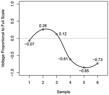
Example 1. Hypothetical audio signal fragment with instantaneous voltage values (relative to digital full scale) for six samples
(click to enlarge)
[2.7] To make the difference between these two methods concrete, consider the hypothetical audio signal fragment shown in Example 1, which consists of six samples taken at equally spaced time points and labeled arbitrarily as 1 through 6 on the x-axis. The y-axis shows the amplitude of the signal, which in the digital domain is a dimensionless quantity representing the ratio of the analog signal voltage entering the digital audio converter to the maximum voltage that the converter can accept before clipping. For the sake of convenience, I will refer to this as the “Voltage Proportional to Full Scale,” with full scale referring to the maximum analog input voltage of the analog-to-digital converter.
[2.8] Let’s now make some RMS calculations with this hypothetical data. For the first three samples, the RMS value would be
For the last three samples, the RMS value would be
If we were to then average (i.e., take the arithmetic mean of) these two individual RMS values to find the overall level of these six samples, we would get
There are so few samples in this hypothetical example, though, that we can easily calculate the RMS level for all six samples directly:
Notice that the average RMS value calculated above (0.4515), which took the arithmetic mean of the RMS level of the first three samples (0.1702) and the last three samples (0.7327), does not equal the true RMS value (0.5319). It is possible, however, to calculate the true RMS value by using the intermediary RMS values derived from the first three and last three samples. To do so, we simply take the RMS of these two RMS values:
As this shows, to determine the overall RMS value of a signal using intermediary RMS values, it’s more accurate to calculate the RMS of those intermediary RMS values, not the arithmetic mean (or average) of those values. For the sake of clarity, I will sometimes refer to the correctly calculated overall RMS value as the “true RMS” value; otherwise, it’s sufficient to simply say the “RMS” value, since it should not be dependent on how the overall result is determined given a particular window of time.
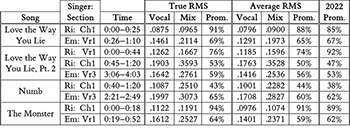
Example 2. Table of true RMS, average RMS, and prominence values for different sections in four collaborations by Eminem (“Em”) and Rihanna (“Ri”)
(click to enlarge)
[2.9] In the example above, the difference between the average RMS value (0.4515) and the true RMS value (0.5319) was derived from only a hypothetical fragment of audio data for the sake of illustration. To what extent, we may wonder, do average RMS values differ from true RMS values when using real-world data? And how might these differences in RMS affect the calculation of prominence? To explore these questions, I recalculated RMS levels and the corresponding prominence scores, using both true RMS and average RMS methods, in the four song collaborations by Eminem and Rihanna that Duguay analyzes in her article. The results are shown in Example 2. To be clear, the data in the “True RMS” and “Average RMS” columns are based on my own re-analysis of each passage from scratch according to the procedure described by Duguay. To do this, I first separated the vocal from the mix of each song section using the Open-Unmix software, then extracted intermediate RMS levels using Jamie Bullock’s RMS amplitude plug-in, and then calculated the overall RMS value. As Example 2 shows, the difference between true RMS and average RMS in the calculation of prominence may be minimal, such as in Rihanna’s first chorus (“Ch1”) from “Numb” (43% versus 44%). In other cases, the discrepancy is larger, reaching a difference of five percentage points, such as in Eminem’s third verse (“Vr3”) from “Numb” (65% versus 60%).
[2.10] For comparison, the values in the rightmost column of Example 2 (labeled “2022 Prom.”) show the prominence values that Duguay reports for each song section in Example 18 of her 2022 article. If my methodology were identical to Duguay’s, the last two columns should match exactly. But despite some trial and error, I was not able to precisely duplicate Duguay’s results. This may be due to a slightly different workflow, such as a different version of the Open-Unmix library (I used v.1.2.1), a different version of Jamie Bullock’s RMS amplitude plug-in (I used v4), or slightly different start or end times for the song sections. Other methodological factors might also be at play. In footnote 25, for example, Duguay mentions that she omitted RMS values lower than 0.02 when calculating the average RMS value for the vocal to avoid including moments of silence or near silence. But I found that my results were closer to Duguay’s when I instead omitted only RMS values lower than 0.002. Nonetheless, I used the threshold of 0.02 that Duguay reports in my calculations shown here.
[2.11] Duguay also implies (in footnote 26) that she did not omit values in the calculation of the average RMS value for the overall mix. I found, however, that not omitting values resulted in prominence scores greater than 100% in some cases, since the mix overall sometimes had a lower average RMS than the isolated vocal (due to the mix having non-trivial spans of time that were significantly quieter than when there was vocal content). As a result, I calculated RMS values (both true and average) for the mix and isolated vocal using only the same time points. In other words, if a time point were dropped in the calculation of the overall RMS value for the isolated vocal, I dropped that same time point in the calculation of the overall RMS value for the mix as well.
[2.12] As the last two columns of Example 2 show, it appears that the calculation of vocal prominence following the workflow outlined by Duguay may vary from user to user. Generally speaking, this variation seems fairly small, usually about two or three percentage points only. The exception is the prominence score for Rihanna’s vocal in the first verse (“Vr1”) of “Love the Way You Lie (Part II),” where Duguay reports a prominence of 92%, whereas I calculated a prominence of only 74% using average RMS. Perhaps a different workflow can in some cases result in a relatively large difference in the prominence score.
[2.13] Overall, Example 2 shows that average RMS values will not give the same results as using true RMS values when working with real-world data. That said, those differences appear to be roughly of the same magnitude as differences based on the particular details of a researcher’s methodology (e.g., slightly different start or end times for a section). Are there ways, then, to ensure a more replicable measurement of prominence? And what do these differences in prominence mean? Is, for example, a 5% swing in prominence audible? More broadly, we might ask: To what extent do prominence values correspond to loudness perception or musical significance? In the next two sections, I address the perceptual interpretation of prominence and provide a workflow that I believe will ensure more consistent results between researchers.
3. Decibels
[3.1] As noted above, Duguay concedes that amplitude is related to but not the same as perceived loudness. Indeed, audio engineers do not typically use RMS amplitude measurements—or ratios of RMS amplitudes—directly as a unit of relative sound level. Instead, the standard practice is to indicate relative sound levels through a logarithmic transformation of amplitude ratios, commonly known as the decibel (Rumsey and McCormick 2021, 16).
[3.2] Most musicians are familiar with the term decibel (or “dB” for short), even if they have never had a reason to manually calculate decibel differences. We will need to understand that calculation here, though, to see the relationship between decibels and prominence. In essence, the decibel measures the ratio of the powers of two signals on a logarithmic scale. More specifically, it can be formulated as
where Pr is the power (in watts) of a reference signal, Ps is the power (in watts) of a signal being compared to that reference, and the coefficient of 10 converts bels into decibels (hence the “deci” prefix). Generally speaking, loudness perception more closely approximates a logarithmic rather than a linear relationship, which is why the formula for the decibel involves a base-10 logarithm. For reference, an increase of 10 decibels (or 1 bel) corresponds roughly to a doubling of perceptual loudness (all else being equal), and a difference of 1 decibel is generally taken to be the “just noticeable difference,” i.e., the minimal amount necessary for the average listener to hear a change in loudness (Thompson 2018, 311–2).
[3.3] We cannot plug RMS amplitude values directly into the decibel equation above, but (as mentioned earlier in paragraph [2.7]) the RMS amplitude in a digital system is proportional to the input voltage on the analog-to-digital converter. This input voltage can be related to power through Ohm’s law, like so:
where P represents the power of the signal (in watts), V represents the voltage of the signal (in volts), and R represents the resistance of the load (in ohms). Assuming a fixed value of R for the two signals we are comparing, we can say that the power of the signal is thus directly proportional to the square of its voltage, i.e.,
Substituting V2 for P in the decibel equation above, we can calculate decibels directly using RMS amplitudes:
where Vr is the RMS amplitude of the reference signal and Vs is the RMS amplitude of the signal being compared to that reference. This formula should be reminiscent of Duguay’s formula for prominence (shown above in [2.1]), which uses a ratio of RMS amplitudes. Unlike Duguay’s formula, though, this formula uses the logarithmic transform of that RMS ratio and a coefficient of 20.
[3.4] Because loudness differences are perceived on a logarithmic scale, I suggest that the operationalization of vocal prominence will better match loudness perception if calculated like so:
where Vs is the (true) RMS amplitude of the isolated vocal and Vr is the (true) RMS amplitude for the other components of the mix. As I will demonstrate below, the output of this equation is more interpretable with regard to the relative level of the vocal in the mix than the output of Duguay’s equation.
[3.5] To be clear, the difference between this formula for prominence and Duguay’s does not involve only the logarithmic transform and multiplication by 20. In addition, the variable Vr in this equation is not the RMS value of the entire mix (which would include the vocal), as it was in the denominator of Duguay’s equation for prominence. Instead, it is the RMS value of the mix without the vocal, i.e., all the remaining non-vocal (or instrumental) components of the mix. This is an important change beyond just the logarithmic transformation of the RMS ratio itself.
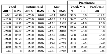
Example 3. Table of different hypothetical levels for vocal, instrumental, and mix, with corresponding prominence calculations using Duguay’s method and the improved method
(click to enlarge)
[3.6] To understand why it’s preferable to compare the vocal to the non-vocal sound sources rather than to the full mix, let’s consider a set of hypothetical examples. In this regard, Example 3 shows various possible combinations of vocal levels, instrumental levels (i.e., the mix without the vocal), and the mix overall. Signal levels are shown in dBFS (more on that in a moment) and true RMS. In the three rightmost columns, the values for vocal prominence have been calculated using: 1) Duguay’s original formula (the “Vocal/Mix %” column); 2) the base-10 logarithmic transform of Duguay’s original formula multiplied by 20 (the penultimate “Vocal/Mix dB” column); and 3) my proposed formula for prominence (the rightmost “Vocal/Inst. dB” column). To be clear, the difference between the last two columns is that the one on the left uses the ratio between the RMS value of the vocal to that of the mix in the decibel equation (shown above in [3.4]), whereas the one on the right uses the ratio between the RMS value of the vocal to that of the instrumental (non-vocal) parts in the decibel equation.
[3.7] In addition to RMS values, signal levels in Example 3 are shown on the dBFS scale, which makes it easier to compare dB levels between signals in the digital domain. The dBFS, which stands for [d]eci[B]els relative to [F]ull [S]cale, is the standard unit of measurement for amplitude levels in a digital system (Thompson 2018, 374). According to the AES17-2020 guidelines set by the Audio Engineering Society (2020), dBFS is defined such that 0 dBFS equals the RMS value of a full-scale sine wave, i.e., a sine wave with an instantaneous positive peak value of 1.000 on a scale of digital amplitude (with no DC offset). Given this peak value, the RMS value for a full-scale sine wave can be found to equal √2/2, or approximately 0.7071. (Showing this calculation is beyond the current scope, as it involves some calculus; see [1998, 26].) As a result, the dBFS value of any digital signal can be determined by using the “20 log” equation for decibels with √2/2 as the RMS value of the reference signal. The dBFS level of a digital signal with an RMS value of 0.1993, for example, can be calculated as follows:
which can be seen in the second row of Example 3 in the “Vocal” column.
[3.8] In Example 3, the level of the instrumental portion of the mix is held constant at -20 dBFS (a common calibration level for digital systems). With the level of the instrumental fixed, different levels of the isolated vocal are shown, which when summed with the instrumental components creates different levels for the mix overall. If, for example, the level of the isolated vocal is -20 dBFS and the level of the instrumental (i.e., the mix without the vocal) is also -20 dBFS, then the level of the mix overall (when the vocal and the non-vocal parts are summed together) would be -17 dBFS. Notice that the RMS levels of the vocal and instrumental components cannot simply be added together to get the RMS level of the mix. In this case, for example, the RMS level of the vocal, 0.707, summed with the RMS level of the instrumental, 0.707, equals 1.000 (not 1.414). This is because the vocal and the instrumental parts are uncorrelated signals, meaning that the frequency and phase components of the signals are independent of one another. When uncorrelated signals are combined (i.e., mixed together), it is the power (not the voltage) of the individual signals that is additive (Hartmann 1998, 42). In other words,
where P represents the power of a particular signal. We don’t have power values for the digital signals in Example 3, but, as we did above, we can substitute the square of voltage (V2) for power (since they are proportional) to get an equation for combining uncorrelated signals in terms of RMS amplitudes:
where V represents the (true) RMS amplitude of a particular signal. To check the validity of this formula using the example above of a vocal and instrumental part at –20 dBFS with an output mix level of -17 dBFS, we can confirm that (0.707)2 + (0.707)2 = (1.000)2 (allowing for rounding error).
[3.9] Now that we have a better understanding of dBFS and how RMS levels of uncorrelated signals combine, let’s take a look at how changes in the level of the vocal are reflected in various ways of measuring vocal prominence. Ideally, a change in the prominence value would be directly interpretable as a change in the level of the vocal relative to the other sound sources in the mix. Everything else being equal, for example, if the vocal level is increased by 9 dB in the mix, the prominence value should also increase by 9 dB, because the vocal is now 9 dB more prominent. This is not, however, what occurs if we simply take the base-10 logarithm of Duguay’s original prominence percentage and multiply it by 20, as shown in the penultimate column in Example 3. Given, for example, a level of -20 dBFS for the instrumental parts of the mix, if the vocal rises from -20 dBFS to -11 dBFS (i.e., a 9 dB gain), plugging Duguay’s prominence percentage into the decibel equation shows only a 2 dB rise (from -3 dB to -1 dB). Notice also that when the vocal and instrumental parts have the same RMS levels (such as when the vocal and instrumental parts are both at -20 dBFS), Duguay’s prominence formula gives a result of 70.7%, which converts to -3 dB. Neither value seems to intuitively convey that the vocal and mix have the same RMS amplitude (i.e., are equally loud).
[3.10] The issue here is that by comparing the level of the vocal to the level of the full mix, Duguay’s original formula partially compares the level of the vocal to itself (since the vocal contributes to the RMS level of the full mix). In contrast, if we take the dB value of the isolated vocal with respect to the instrumental (non-vocal) portions of the mix, we can more faithfully represent level changes in the vocal part, as shown in the rightmost column of Example 3. When the vocal and non-vocal parts have equal RMS levels, the prominence value becomes 0.0 dB (which corresponds to no difference in level). When the RMS level of the vocal is 9 dB more than the RMS level of the instrumental components, the prominence value becomes +9 dB. And so on. Notice that comparing the RMS level of the vocal to the instrumental (as shown in the “Vocal/Inst.” column) is especially better at representing changes in vocal prominence (as shown in the “Vocal dBFS” column) when the vocal is louder than the mix, i.e., when the vocal is actually prominent.
[3.11] As Duguay mentions ([3.7]), the Open-Unmix software separates the original source into four components: bass, drums, vocal, and “other.” It does not, in other words, separate the signal into a vocal component and a second audio file for everything else (i.e., the instrumental, non-vocal portion of the mix). It may, therefore, appear that we cannot determine the RMS level of the instrumental parts given a real-world audio recording. But is not difficult to calculate the RMS level of the instrumental parts if we know the RMS level of the isolated vocal and the mix overall. Given that the isolated vocal and instrumental parts are uncorrelated signals, we can use the formula above for combining the RMS levels of uncorrelated signals and solve for the unknown, like so:
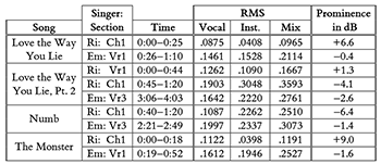
Example 4. Recalculation of vocal prominence in terms of decibels (dB) for four collaborations by Eminem (“Em”) and Rihanna (“Ri”), as analyzed by Duguay (in Example 18)
(click to enlarge)
[3.12] Using this technique, I recalculated the relative level of the vocal for the four Eminem and Rihanna collaborations that Duguay discusses. This data is shown in Example 4, which recasts that portion of Example 18 in Duguay’s article. The dB level in the rightmost column corresponds to prominence calculated according to the method using the enhancements discussed thus far, which compares the (true) RMS level of the isolated vocal to the (true) RMS level of the instrumental. As a reminder, the RMS levels for the vocal and mix overall are my own calculations using my own data, which may differ slightly from those found by Duguay (as discussed previously in [2.10–2.12]).
[3.13] To be clear, producing data such as that shown in Example 4 requires a great deal of effort and manual computation. After editing each song to create audio files for each individual section and then isolating the vocal track as its own file, I loaded each audio file into Sonic Visualiser to generate a list of RMS values. I then imported these lists of RMS values into Microsoft Excel to calculate the (true) overall RMS values, filtering out any timepoints of silence in the vocal part and the corresponding timepoints in the mix. After that, I used Excel to calculate the level of the instrumental parts, from which I could finally plug RMS levels into the decibel equation to get the prominence value for each section in dB. Given that there were challenges with regard to replicability for prominence using Duguay’s original formula (as discussed above in [2.10–2.12]), it is unfortunate that the enhancements proposed thus far come at the cost of increased computational complexity (and thus, presumably, an increase in the potential for user error). In the next and last stage of enhancement, discussed below, I thus offer a simplified workflow for measuring prominence as well as a final improvement to even better model the relationship of prominence to loudness perception.
4. Loudness Units
[4.1] As explained in [3.2] above, the unit of the decibel is defined as the ratio of the power of two signals on a logarithmic scale. The decibel maps fairly well to loudness perception; better, say, than this same power ratio expressed on a linear scale. But decibel measurements based on raw RMS signal levels do not account for the non-linear response of the human ear to different frequencies at different sound pressure levels.
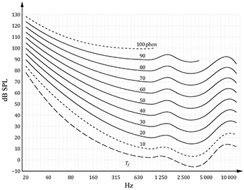
Example 5. Equal-loudness-level contours for pure tones under free-field listening conditions (ISO 226:2023). The long-dashed line indicates the threshold of hearing (Tf). Contour lines at 10 and 100 phons are drawn with short-dashed lines due to a lack of sufficient experimental data
(click to enlarge)
[4.2] The sensitivity of the human ear to different frequencies at different sound pressure levels is typically represented as a set of equal-loudness-level contour lines, dating back most famously to the work of Fletcher and Munson (1933). The latest data is shown in Example 5, which displays the equal-loudness-level contours released by the International Organization for Standardization (ISO) in their 2023 report (226). In this graph, the x-axis represents frequency (on a logarithmic scale) in the units of hertz (Hz), and the y-axis represents acoustical sound pressure level (as dB SPL), which is a ratio of the atmospheric pressure change in pascals (Pa) to the reference level change of 20 μPa (0 dB SPL, also known as the absolute threshold of hearing).
[4.3] Each contour line in the Example 5 traces a particular level of phon, which is the logarithmic unit of loudness (as compared to the sone, which is the linear unit of loudness). More specifically, each contour line is defined as the dB SPL level at a given frequency that is perceptually equivalent to a pure 1 kHz tone at some particular level in dB SPL. For instance, to be the same loudness as a 1 kHz tone at 40 dB SPL (the 40 phon contour line), a 40 Hz tone—which is roughly the fundamental frequency of the low E string on the bass guitar—would need to be about 83 dB SPL. Notice that the human ear is particularly sensitive to frequencies in the range of about 2 kHz to 5 kHz, where each contour line dips down, but much less sensitive to higher and (especially) lower frequencies.
[4.4] Notice also that the contour curves in Example 5 are not equally spaced at all frequencies. In particular, the equal-loudness-level curves get more tightly spaced at lower frequencies. To be as loud as a 1 kHz tone at 80 dB SPL (the 80 phon contour), that 40 Hz of the low E string would have to be only about 105 dB SPL, a much smaller dB difference than seen in the 40 phon contour. Generally speaking, the frequency response of the human ear flattens out with an increase in overall level. Listening to music at lower playback volumes, therefore, will result in an especially significant lack of bass and high end.
[4.5] To account for the uneven sensitivity of the human ear to different frequencies at difference sound pressure levels, we can imagine applying equalization to the music before assessing its overall loudness, raising certain frequencies and attenuating others. This applied equalization would ideally be the inverse of the equal-loudness-level contours, decreasing the level of lower frequencies in the mix and raising frequencies in the range of 2 kHz to 5 kHz, since our ears are less sensitive to lower frequencies and more sensitive to frequencies in the upper midrange.
[4.6] Because these equal-loudness-level contours are not equally spaced, however, there is no single equalization curve that can account for all possible listening levels. Accordingly, a variety of different frequency weighting curves have been proposed, such as A-weighting (which was designed to be the inverse of the equal-loudness-level contour line at 40 phons), B-weighting (the inverse of the contour line at 70 phons), C-weighting (the inverse of the contour line at 100 phons), and so on. In a recent paper, for example, Skovenborg and Nielsen evaluate twelve different weighting schemes meant to model loudness perception (2004).
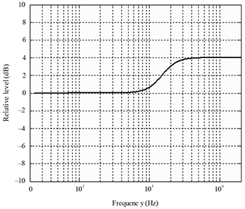
Example 6. Frequency response of high-shelf filter used in the first stage of K-weighting (ITU-R BS.1770-4)
(click to enlarge)
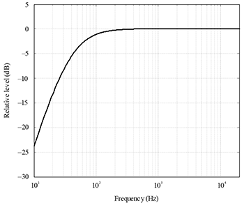
Example 7. Frequency response of high-pass filter used in the second stage of K-weighting (ITU-R BS.1770-4)
(click to enlarge)
[4.7] But while many different equalization weighting schemes have been proposed, K-weighting has become the current standard, as outlined in recommendation ITU-R BS.1770-4 by the International Telecommunication Union (BS.1770-4) and in recommendation EBU R-128 by the European Broadcast Union (2020). K-weighting consists of two filters applied to the audio signal that account for the uneven sensitivity of the human ear to different frequencies. The first stage, as shown in Example 6, is a second-order high-shelf filter, with 4 dB of gain and a cutoff frequency of about 1.7 kHz. In essence, this first-stage filter models the increased sensitivity of the human ear to upper midrange frequencies (i.e., those between 2 kHz and 5 kHz) by boosting their level. The second stage, as shown in Example 7, is a second-order high-pass filter with a cutoff frequency of about 60 Hz. In essence, this second-stage filter models the ear’s lack of sensitivity to lower (bass) frequencies by reducing their level. Admittedly, the combination of these two filters does not create an exact inverse of any of the equal-loudness-level contour lines. But it’s a “good enough” approximation that has, for better or worse, become the current recommended standard for measuring loudness (Thompson 2018, 381–2).
[4.8] When audio is K-weighted with these two filters, loudness in the digital domain is measured not on the dBFS scale but rather on the LUFS scale, which stands for [L]oudness [U]nits relative to [F]ull [S]cale (Brixen 2020, 68). Differences on the LUFS scale are measured in terms of Loudness Units, or LUs, with 1 LU = 1 dB. That is, the LUFS scale is the same as the dBFS scale, except with the understanding that the audio has been pre-processed using loudness-based weighting equalization prior to taking RMS amplitude measurements and then being logarithmically transformed by the decibel equation. To be clear, the LUFS scale is theoretically independent of any particular weighting scheme. It is generally assumed, though, that LUFS measurements currently use the K-weighting standard unless specified otherwise.
[4.9] To calculate vocal prominence, therefore, we could compensate for the unequal frequency response of the ear at difference sound pressure levels by pre-processing the audio files with equalization that applies K-weighting (prior to taking RMS measurements and then calculating dBFS and relative dB levels). That’s not impossible to do manually, but this additional step would add yet another stage in what is already a fairly complex workflow for determining prominence. Thankfully, high-quality loudness meters are available that will implement this workflow automatically. One free version (with the option for a paid upgrade) is the Youlean Loudness Meter; similar meters for purchase are available from iZotope (Insight 2), Waves (WLM Plus), and others. In essence, these loudness meters first apply K-weighting to the audio file, then take momentary amplitude measurements of this weighted audio to calculate an overall RMS level, and finally transform these RMS measurements to a logarithmic scale through the decibel equation. The result is a measure of loudness on the LUFS scale. In particular, the Integrated Loudness display on these meters (sometimes labeled as the “Long Term” loudness) indicates the overall loudness for the entire playback window of the audio file.
[4.10] As an added benefit, loudness meters also automatically compensate for moments of silence in the audio file that might otherwise skew the overall loudness value. Recall that Duguay accounted for passages of silence by omitting RMS amplitude values below 0.02. In a loudness meter, moments of silence are removed through the use of two gates (as detailed in ITU-R BS.1770-4). The first gate is absolute and has a fixed threshold of -70 LUFS; no audio below this level is included in the overall calculation. (For comparison, Duguay’s reported RMS threshold of 0.02 corresponds to about -34 dBFS.) The second gate is relative, with a moving threshold of -10 dB (or LU) based on the current overall LUFS value.
[4.11] A loudness meter thus offers an all-in-one assessment of loudness (and thus prominence) with minimal manual calculations. That said, there is one final aspect of determining prominence using a loudness meter that still needs to be addressed. As detailed in the previous section, I recommended that prominence be measured not between the vocal and the full mix but instead between the vocal and the mix minus the vocal. Yet the Open-Unmix software does not isolate the mix without the vocal (in contrast to some non-free software, such as iZotope RX, that will). My workaround in Example 4 was to calculate the RMS levels of the mix minus the vocal using mathematical methods based on how the powers of uncorrelated signals combine. There was value in illustrating this process, yet it would be preferable if we could measure the loudness of the mix minus the vocal directly.
[4.12] Fortunately, an audio file of the mix minus the vocal can be created easily using most digital audio editors. To do so, first align the beginning of the isolated vocal track with the beginning of the full mix. Then, reverse the polarity of the isolated vocal track so that it cancels out this content in the full mix. If the two tracks are at unity gain (i.e., no changes in level have been made), then when the polarity-reversed isolated vocal track is mixed with the original track, the output will be the full track without the vocal.
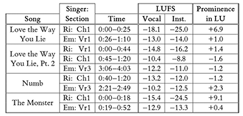
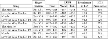
Example 8. Recalculation of vocal prominence in terms of loudness units (LU) for four collaborations by Eminem (“Em”) and Rihanna (“Ri”), as analyzed by Duguay (in Example 18)
(click to enlarge)
[4.13] Using this procedure, I recalculated vocal prominence in terms of LU for the nine musical excerpts analyzed by Duguay in Example 18 of her article. This data is shown below in Example 8. Notice that these prominence values are similar to those shown previously in Example 4 but not identical. As we should expect, the prominence values in LU (shown here) are consistently higher than the prominence values in dB (shown in Example 4), since the K-weighting emphasizes frequencies within the typical range of a vocal (such as the upper midrange) and de-emphasizes frequencies outside this range (such as the bass).
[4.14] To summarize, the workflow I am ultimately proposing for calculating prominence is:
- Edit the audio file of the original song to span only the passage over which prominence is to be calculated.
- Import the edited audio file of the full mix into software (such as Open-Unmix) that will extract the vocal from the mix as a separate audio file.
- Create an audio file of the mix minus the vocal by canceling out the vocal from the mix using polarity reversal (or another method).
- Using a loudness meter, determine the integrated loudness level in LUFS for the isolated vocal as well as the mix minus the vocal.
- Calculate the prominence of the vocal in LU by subtracting the integrated LUFS level of the mix minus the vocal from the integrated LUFS level of the isolated vocal.
Although this workflow describes how to calculate the prominence of a vocal with respect to the mix, it could also be used to calculate the prominence of any other track in a mix (assuming it can be isolated as a separate audio file), such as the bass, guitars, or drums. It could also be used to compare the relative loudness of one element of the mix to another, such as the vocal to the bass or the drums to the guitars.
5. Conclusion
[5.1] As outlined above, the method for measuring prominence that I am proposing provides what I believe to be a more accurate and perceptually meaningful value for assessing the relative loudness of the vocal to the rest of the mix. It also reduces the amount of computation involved, thus hopefully ensuring more consistent results between researchers. That said, the reader may nonetheless wonder what (if any) effect these enhancements have on the analysis of music. To what extent, in other words, does this improved formulation of prominence translate to improved musical insights? I’ll address this question from two perspectives: the first involving a re-analysis of the four songs that Duguay examines in her article, the second involving a consideration of prominence within visualizations of three-dimensional virtual space.
[5.2] In her analysis of the four collaborative tracks by Eminem and Rihanna, Duguay attributes differences in vocal prominence to differences in gender (as she suggests in [1.7] and [4.10]). At the end of her article ([4.6]), Duguay concludes (based on her calculations of vocal prominence) that Rihanna’s voice “takes on a prominent role in comparison to the other sound sources heard in the mix,” whereas Eminem’s voice is “more blended within the virtual space.” This seems to somewhat hold true for these four songs, but there may also be confounding variables.
Example 9. Vocal prominence in terms of loudness units (LU) for four collaborations by Eminem (“Em”) and Rihanna (“Ri”), ordered by decreasing prominence
(click to enlarge)
[5.3] For instance, Example 9 reorders the data from Example 8 with respect to decreasing vocal prominence as measured in LU. (The tiebreaker for the rows with a prominence of -1.2 LU was the prominence in dB; see Example 4.) For comparison, the last column in Example 9 (“2022 Prominence”) shows the original prominence values calculated by Duguay. Notice, first of all, that vocal prominence tends in most cases to be within one or two LU of zero LU, plus or minus. That is, the vocal is typically about as loud as the rest of the mix, given that 1 dB (or 1 LU) is the just noticeable difference for perceptual loudness.
[5.4] The notable exceptions are the data points in the first two rows, where Rihanna’s vocal is +9.1 dB and +6.9 dB more prominent than the rest of the mix. Notice, however, that these two cases both occur within an introductory chorus section (with a start time of 0:00). Generally speaking, it appears that vocal prominence in these nine musical passages has some correlation with the specific role of that section in the song. Vocal prominence is lowest, for example, in the two internal chorus sections (the bottom two rows of Example 9), presumably due in part to these passages having a particularly dense and thick instrumental texture, as is typical of a main (non-intro) chorus. Vocal prominence values for the verse sections are in between these extremes, which makes sense since the instrumental texture of a verse is usually less dense than a full-blown chorus but typically more dense than an intro. To be fair, the data here is limited, and these differences are typically on the order of only a few dB above or below zero LU. The main observation from this data, perhaps, is that mix engineers tend to balance the level of the vocal with the rest of the mix, regardless of other factors.
[5.5] Stepping back, the reader may wonder what implications my recommendations have on visualizations of vocal placement in the virtual space of a sound recording. That is, after all, a central goal of Duguay’s article, in which recorded virtual space is represented as a rectangular cuboid. In Duguay’s conceptualization, prominence is plotted on the depth axis of this virtual space ([3.13])—i.e., on the dimension between the front and back faces (or “walls”) of the rectangular cuboid—with the front wall corresponding to 100% prominence (a vocal with no mix) and the back wall corresponding to 0% prominence (a mix with no vocal). Differences in prominence percentages are represented as linear distances along this depth axis. A prominence value of 70.7%, for example (which represents an equal vocal level with the mix; see Example 3), would thus be seven-tenths of the distance from the back wall to the front. Duguay argues at length for this approach ([3.15–3.18]), in which the depth axis of a virtual space is based on amplitude alone rather than considering other factors such as timbre or time-based effects. One of Duguay’s main points is that modern sound recordings do not necessarily mimic natural spaces, so there is no consistent relationship between, say, the amount of reverb on a vocal and its location in a virtual space. More practically, her approach makes it easier to quantify the depth axis instead of relying on subjective assessments of distance.
[5.6] I think Duguay’s reduction of the depth axis to amplitude alone is reasonable, if only to serve as an objective mechanism for plotting the closer-to-farther sensation of sources in a mix. Rather than scaling the depth axis of prominence in terms of percentages, as Duguay does, we can scale it instead in terms of LU. This may seem impossible, given that LU and dB values are theoretically boundless. The prominence of a mix without a vocal, for example, would ideally correspond to a dB value of negative infinity (see Example 3), and the prominence of a vocal without a mix would ideally correspond to a dB value of positive infinity (as the limit of the RMS value of the mix approaches zero). But since every real-world sound recording has some non-zero noise floor, real-world prominence values will inherently be bounded. Moreover, if we are interested in analyzing the non-trivial cases of when a musical passage includes both vocal and instrumental content, prominence values will typically lie within a fairly narrow range of LU values. Looking back at Example 9, for instance, prominence values as measured in LU all fall between –2 LU and +10 LU. I would thus suggest that—if a researcher is interested in visualizing prominence within a virtual space—the halfway point of the depth axis should be set to 0 LU, which represents an equal loudness between vocal and mix, and the front and back walls should be set to whatever equidistant LU levels are sufficient to capture a useful range. Perhaps with more research on typical prominence values across musical styles, the LU levels of the front and back walls could be standardized. I would estimate that a range of 20 LU (from –10 LU to +10 LU) would cover most cases, and a range of 40 LU (from –20 LU to +20 LU) would cover almost all cases. Any particularly extreme values could be subsumed within the axis boundaries, as is commonly done with other visualizations that involve logarithmic scales (e.g., polar pattern plots of microphone directional sensitivity, in which the center point will subsume all values from –30 dB to negative infinity dB). Alternatively, a researcher could map the depth axis of the three-dimensional virtual space not to prominence but rather to absolute LUFS values, with the front wall at 0 LUFS and the back wall at some acceptable negative LUFS value, to show loudness relationships between various sources within the mix.
[5.7] I look forward, therefore, to music researchers more broadly investigating the relationship of the vocal to other instruments in the mix. In this regard, the enhancements I have offered here are intended to facilitate not only a less computationally intensive workflow for quantifying prominence but also more accurate measurements that better match human perception and modern audio engineering practices. I expect that future work will offer yet further improvements to the operationalization of vocal prominence—as well as other aspects related to the virtual space of sound recording—since research in music theory beyond the traditional domains of rhythm and pitch is still relatively nascent. In that regard, I want to thank Duguay for leading the field in this direction, and I hope that she and other scholars continue this important work.
Trevor de Clercq
Middle Tennessee State University
Department of Recording Industry
1301 East Main Street, MTSU Box 21
Murfreesboro, TN 37132
tdeclercq@mtsu.edu
Works Cited
Audio Engineering Society. 2020. “AES17-2020: AES Standard Method for Digital Audio Engineering: Measurement of Digital Audio Equipment.” https://www.aes.org/publications/standards/search.cfm?docID=21.
Aldrich, Nika. 2005. Digital Audio Explained for the Audio Engineer. 2nd ed. Sweetwater Sound.
Ballou, Glen, ed. 2015. Handbook for Sound Engineers. 5th ed. Focal Press. https://doi.org/10.4324/9780203758281.
Brixen, Eddy. 2020. Audio Metering: Measurements, Standards, and Practice. 3rd ed. Focal Press. https://doi.org/10.4324/9781315694153.
Corey, Jason, and David Benson. 2017. Audio Production and Critical Listening. 2nd ed. Routledge. https://doi.org/10.4324/9781315727813.
Duguay, Michèle. 2022. “Analyzing Vocal Placement in Recorded Virtual Space.” Music Theory Online 28 (4). https://doi.org/10.30535/mto.28.4.1.
European Broadcast Union. 2020. “EBU R128: Loudness Normalisation and Permitted Maximum Level of Audio Signals.” https://tech.ebu.ch/docs/r/r128.pdf.
Fletcher, Harvey, and W.A. Munson. 1933. “Loudness, Its Definition, Measurement and Calculation.” Journal of the Acoustical Society of America 5: 82–108. https://doi.org/10.1121/1.1915637.
Hartmann, William M. 1998. Signals, Sound, and Sensation. Springer.
Howard, David, and Jamie Angus. 2017. Acoustics and Psychoacoustics: Technical Ear Training. 5th ed. Focal Press. https://doi.org/10.4324/9781315716879.
International Organization for Standardization. 2023. “ISO 226:2023 Acoustics: Normal Equal-Loudness-Level Contours.”
International Telecommunication Union. 2015. “ITU-R BS.1770-4 Algorithms to Measure Audio Programme Loudness and True-Peak Audio Level.” https://www.itu.int/rec/R-REC-BS.1770.
Pohlmann, Ken. 2011. Principles of Digital Audio. 6th ed. McGraw Hill.
Rumsey, Francis, and Tim McCormick. 2021. Sound and Recording: Applications and Theory. 8th ed. Routledge. https://doi.org/10.4324/9781003092919.
Self, Douglas, ed. 2010. Audio Engineering Explained. Focal Press.
Skovenborg, Esben, and Søren Nielsen. 2004. “Evaluation of Different Loudness Models with Music and Speech Material.” In Proceedings of the 117th Convention of the Audio Engineering Society, Berlin, May 8–11. http://www.aes.org/e-lib/browse.cfm?elib=12770.
Stöter, Fabian-Robert, Stefan Uhlich, Antoine Liutkus, and Yuki Mitsufuji. 2019. “Open-Unmix: A Reference Implementation for Music Source Separation.” Journal of Open Source Software 4 (41). https://doi.org/10.21105/joss.01667.
Thompson, Dan. 2018. Understanding Audio: Getting the Most Out of Your Project or Professional Recording Studio. 2nd ed. Berklee Press.
Watkinson, John. 2001. The Art of Digital Audio. 3rd ed. Focal Press.
Footnotes
1. For those interested in an overview of audio fundamentals, I recommend Thompson (2018); for those interested in learning more about the technical side of audio engineering, I recommend Self (2010), Ballou (2015), and Rumsey and McCormick (2021); for those interested in learning more about digital audio technology in particular, I recommend Watkinson (2001), Aldrich (2005), and Pohlmann (2011); and for those interested in learning more about psychoacoustics, metering, and audio measurement, I recommend Howard and Angus (2017), Corey (2017), and Brixen (2020).
Return to text
Copyright Statement
Copyright © 2024 by the Society for Music Theory. All rights reserved.
[1] Copyrights for individual items published in Music Theory Online (MTO) are held by their authors. Items appearing in MTO may be saved and stored in electronic or paper form, and may be shared among individuals for purposes of scholarly research or discussion, but may not be republished in any form, electronic or print, without prior, written permission from the author(s), and advance notification of the editors of MTO.
[2] Any redistributed form of items published in MTO must include the following information in a form appropriate to the medium in which the items are to appear:
This item appeared in Music Theory Online in [VOLUME #, ISSUE #] on [DAY/MONTH/YEAR]. It was authored by [FULL NAME, EMAIL ADDRESS], with whose written permission it is reprinted here.
[3] Libraries may archive issues of MTO in electronic or paper form for public access so long as each issue is stored in its entirety, and no access fee is charged. Exceptions to these requirements must be approved in writing by the editors of MTO, who will act in accordance with the decisions of the Society for Music Theory.
This document and all portions thereof are protected by U.S. and international copyright laws. Material contained herein may be copied and/or distributed for research purposes only.

Prepared by Andrew Eason, Senior Editorial Assistant
Number of visits:
624