Review of Jason Yust, Organized Time: Rhythm, Tonality, and Form (Oxford University Press, 2018)
Leah Frederick
KEYWORDS: Yust, time, graph theory, hierarchy, syncopation, sonata form, Lewin, non-commutative GIS
DOI: 10.30535/mto.26.4.11
Copyright © 2020 Society for Music Theory
[1] If one were to construct a map of the field of music theory, three of its most prominent regions would represent the subdisciplines of rhythm and meter, tonal structure, and form. One could imagine a number of winding trails on this map, each representing the trajectory of an individual piece of scholarship. Though each path would represent a unique journey, many would explore the local highlights of only a single region, reflecting the tendency for theorists to focus on the way a single musical parameter functions within the works of a particular composer, style, or genre. If drawn on such a map, the trek representing Jason Yust’s Organized Time: Rhythm, Tonality, and Form (2018) would trace out a fundamentally different shape: not only would it visit all three regions, but it would also wind through the stretches of land between them, allowing its travelers to appreciate how the views evolve along the journey.
[2] Organized Time also opens with a map, though not of the imaginary landscape described above. Yust’s map depicts an actual stretch of the Washington State coastline, specifically highlighting several possible sightlines that one might encounter while on the hike from Third Beach to Toleak Point, two prominent locations on the beach. Yust uses this imagery to invoke our temporal experience of music:
This book is about musical landscapes, those created by relationships between durations (rhythm), pitches and harmonies (tonality), and melodic motives and ideas (form). While listening to music we traverse these musical landscapes, and as we listen we look ahead, just as we do while walking the beach, seeing proximate and more distant goals, and some of those in between. (3)
This metaphor ultimately serves to introduce Organized Time’s concept of a temporal structure. Although the beach exists as an atemporal object, the journey along it temporalizes that physical space into a set of locations with a definite ordering in time. Musical structure is likewise made up of events arranged in time, although such musical events belong to different modalities.(1) In tonal music, the ordering of chords is arranged according to hierarchical principles of harmonic syntax, whereas the ordering of rhythms exists within a separate hierarchical framework, that of meter. Yust argues that the events within any single musical dimension—rhythm, tonality, or form—can be arranged into a hierarchical temporal structure.(2) This idea leads to two central premises of Organized Time: first, that the temporal structures of these three musical dimensions are fundamentally independent, and, second, that the most interesting phenomena in tonal music arise from interactions between these different modalities. In the process of disentangling these musical dimensions, Yust reconciles his approach with many of music theory’s cornerstones, including theories of rhythm and meter, Schenkerian analysis, and scholarship of the “new Formenlehre.”
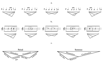
Example 1. Temporal structures (MOPs)
(click to enlarge)
[3] What ties together this immense undertaking is another key observation: the formal (i.e., mathematical) properties of temporal structure are the same in any musical dimension. This allows Yust to develop a single theoretical tool, a type of mathematical graph called a maximal outerplanar graph, abbreviated “MOP,” to represent temporal structures in all three dimensions.(3) In mathematics, discrete graphs are sets of vertices connected by edges; in Yust’s application, the vertices represent timepoints of musical events and the edges represent timespans. Example 1 depicts some simple applications of MOPs in the rhythmic, tonal, and formal domains. In all of these graphs, the horizontal edge along the top, called the root, represents the timespan of the entire excerpt. The first node one level down, which creates the uppermost inverted triangle in the graph, divides the longest timespan into two shorter ones.(4) In the example, these shorter timespans represent different things in each modality: the duration of a half note (Example 1a);(5) the Urlinie motion from – and – (Example 1b); or the antecedent-consequent and presentation-continuation sections of small formal structures (Example 1c).(6) After this first division, subsequent nodes can be added to divide the left or right edges, adding depth and creating graphs with different abstract shapes.
[4] Although this theoretical agenda serves as the underlying framework for Organized Time, Yust channels his analytical observations to construct a narrative about eighteenth-century style and the development of sonata form. Woven into theories concerning hypermeter, counterpoint, and tonal-formal disjunction are arguments about the stylistic traits of individual composers, such as those characterizing Boccherini’s normative approach to formal structure in his sonatas (85), Haydn’s use of hypermetrical techniques to create cadences with differing amounts of closure in his symphonic expositions (133–40, 159–62), Mozart’s experimentation with the misalignment of rhythmic and formal structures in several works from the year 1788 (151–58), Beethoven’s delay of full rhythmic-tonal closure until after the exposition in his middle-period works (170–76), and Galuppi’s formal “recipe” for his keyboard sonatas (283–87). As this list suggests, Organized Time contains analyses not only of works by canonic figures, but also of gems by numerous other lesser-known eighteenth-century composers.(7) Yust’s rationale for drawing on repertoire outside of the canon is tied to the larger project at hand: he argues that the field’s focus on only canonic composers limits the ways that we theorize, in particular, about the interactions between form and tonality.(8)
[5] The scope of musical excerpts discussed in Organized Time ranges from a few measures to entire movements. Beautifully produced scores appear on nearly every page of the book, and most of these figures also incorporate detailed text and graphical annotations. Though there are places where Yust comments on sections or pieces that are not included in the examples, readers can verify the majority of his analytical claims from the examples provided. Examples 2 and 3 depict portions of Yust’s analysis of the first movement of Beethoven’s String Quartet in F minor, op. 95 (“Serioso”). This analysis appears at the end of chapter 8, on syncopation, as evidence for the section’s thesis that, in Beethoven’s music, “rhythmic irregularities often take on more pervasive thematic, motivic, and formal significance” (191). In addition to capturing the general nature and visual layout of Organized Time’s more extended analyses, this example provides a glimpse into how the theoretical insights accumulated in prior chapters—here, those concerning syncopated rhythmic structure—culminate a compelling, movement-long analysis.
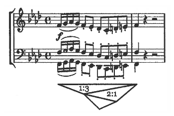
Example 2. Syncopated rhythmic structure in the opening of Beethoven’s String Quartet in F minor, op. 95
(click to enlarge)
[6] The rhythmic structure of the String Quartet’s opening gesture is represented by the MOP shown in Example 2. Though the surface rhythms of this passage do not appear to be syncopated, Yust justifies his interpretation by citing the unison motive’s contour, articulation, and scalar inflections (196–97). The syncopation is conveyed in the MOP by the labeled timespan ratios, 1:3 and 2:1, which compare the uneven timespan lengths of this syncopated rhythm to the more even timespans of a “normative rhythm.” The 1:3 timespan ratio signifies that the measure-long timespan divides into 
 .| |. also divides unevenly, so that it breaks into |. .|
[7] This understanding of the syncopated rhythm as deriving from a similar, but more even, version of the same rhythm illustrates Yust’s general approach to rhythmic structure. As introduced in chapter 1, a collection of rhythms that share the same hierarchical structure (or, equivalently, MOP network representation) is known as a rhythmic class.(10) The normative rhythm is “the most regular representative of the given class” (16). By expanding and contracting the timespan lengths within a normative rhythm, one can generate an entire family of related rhythms. Syncopations arise as a specific type of such timespan adjustments, one that “pairs an expansion with a compensating contraction elsewhere in the hierarchy” (121). Though they appear in the MOPs as simple integer ratios, we learn in chapter 5 that these expansions and contractions actually exist within a generalized interval system of timespan transformations proposed by David Lewin, on which more below.
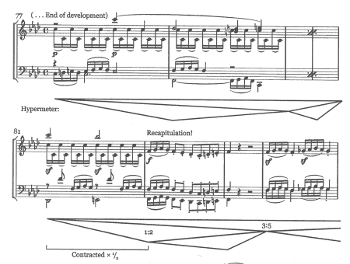
Example 3. Analysis of Beethoven’s String Quartet in F minor, op. 95, mm. 77–88 (Organized Time, Example 8.17)
(click to enlarge and see the rest)
[8] The presence of this syncopation in the Quartet’s initial measure foreshadows its motivic significance later on in the movement. Yust details three subsequent passages featuring notable syncopations: the cadential section of the subordinate theme, the juncture between development and recapitulation, and the beginning of the coda. Example 3 shows the second of these, which also happens to be the most illustrative, as it testifies to Organized Time’s overarching thesis.
[9] In the first system of Example 3a, the evenness of the MOP conveys a regular two-bar hypermeter at the end of the movement’s development. (Chapter 6 extends this timespan approach to rhythmic structure to the hypermetrical level.) New hypermetrical units at the 2- and 4-bar levels begin at the start of the second system (m. 81), but the unexpected appearance of the Quartet’s dramatic opening interrupts, disturbing this steady hypermetrical pattern. This ultimately results in large-scale syncopation, as an expansion in mm. 86–88 compensates for m. 81’s contraction. Example 3b shrinks the hypermetrical MOP from Example 3a in order to present it alongside a corresponding MOP depicting the excerpt’s formal structure. Comparison of the two MOPs shows that the hypermetric syncopation (mm. 81–89) occurs alongside the recapitulation’s fused main theme and transition sections, though misaligned by a measure. Thus, as evidence for the book’s central hypothesis, this hypermetrical syncopation coincides precisely with the critical moment of recapitulation, revealing a large-scale disjunction between the modalities of rhythm and form.
[10] While MOPs appear alongside the majority of the book’s musical examples, Yust’s analytical commentary largely avoids explicit mention of them. After their uses are introduced in the rhythmic, tonal, and formal domains (chapters 1–3), the graphs most often serve as an efficient visual mechanism by which to communicate Yust’s analytical interpretations of individual pieces. Since the prose centers around the music, not the graphs, Organized Time remains accessible to a wide audience. Though the book does demand familiarity with the standard literature of the field, its contents are so varied and plentiful that it likely contains something of interest to nearly anyone who studies musical structure. One topic that will undoubtedly draw future attention is Yust’s novel approach to form, which in itself could be the subject of another monograph.(11) The proposal of independent modalities entails that the theory of formal structure, developed in chapters 3 and 11, must be completely independent of tonal entities, both local harmonic progressions and global key areas. This implication leads to a fascinating re-invention centered around four main features—repetition, contrast, fragmentation, and caesuras—and motivates Yust to interrogate the very essence of what it means to construct a “theory of form.”(12) These ideas lead to further questions—e.g., What does it mean for “counterpoint” to exist between formal structures? (225–31)—and to an original conception of form that is ripe for extension to other kinds of music, including post-tonal repertoires.
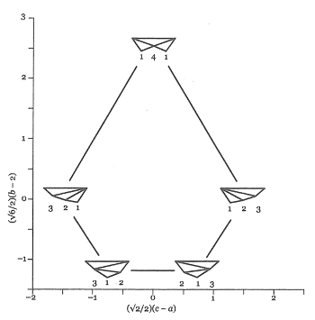
Example 4. The 3-associahedron relating the all possible 3-MOPs from Example 1
(click to enlarge)
[11] Mathematically curious readers will inevitably find themselves with questions about the abstract structure of MOPs as mathematical graphs.(13) Answers to those questions are initially addressed in chapter 4, which constructs machinery for enumerating MOPs; provides ways of measuring depth, distance, and evenness in the graphs; and introduces terminology for classifying different structures.(14) A rigorous mathematical presentation is withheld until chapter 13, which situates the MOP networks within the mathematical subfield of graph theory and demonstrates their relationship to Lerdahl and Jackendoff’s (1983) prolongational trees.(15) The final chapter, chapter 14, proposes a way to compare all possible n-MOPs using a kind of geometric object called an associahedron, formally an (n–1)-dimensional polytope. The 3-associahedron shown in Example 4 translates all five 3-MOPs (from Example 1) into (x, y, z) points and plots them in a three-dimensional coordinate system.(16) Since all five points lie in the same plane of the space, this associahedron is a two-dimensional pentagon. Representing larger MOPs requires more dimensions, and Yust employs several elegant projections of a four-dimensional associahedron in conjunction with analyses of tonal-formal disjunctions in works by Haydn and Schubert (384–87). Within the trajectory of the entire book, these associahedra serve as a culmination of the graph-theoretic formalism that ties back into Organized Time’s central claim: since MOPs with different structures are represented by different points in the space, disjunctions between musical modalities can be captured as distances between vertices of the associahedra.
Example 5. Lewin’s Timespan Interval GIS
(click to enlarge and see the rest)
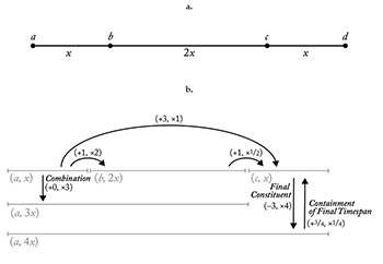
[12] I would like to draw attention to one rather brief section of Organized Time that might easily go unappreciated amidst this landscape of big ideas: Yust’s application of David Lewin’s non-commutative generalized interval system (Example 5).(17) This system is particularly well-suited for comparing timespans within different hierarchical levels since, rather than comparing timespans to a fixed unit of time, it measures them relative to each another. Yust largely downplays the role of the timespans within Lewin’s transformational framework—likely an intentional decision, since the intricacies of the non-commutative GIS are not directly relevant to his subsequent chapters. But understanding how these timespan intervals are situated within the more general context of the non-commutative GIS, as I endeavor to show below, both highlights the novelty of Yust’s application and celebrates the inherent elegance of Lewin’s system.
[13] The relationship between any pair of timespans can be captured using a timespan interval (+n, ×m), which compares the timespans based on their starting points and lengths. Suppose one timespan, called (a, x), begins at timepoint a and lasts for duration x, and another, (b, y), begins at timepoint b and lasts for duration y. If (+n, ×m) is the timespan interval from (a, x) to (b, y), then +n in the timespan interval measures the starting point of the second interval (b, y) in units relative to the first timespan—that is, in lengths of x. Likewise, ×m measures the length of (b, y) as a proportion of x. Example 5a depicts a timespan divided into a short-long-short pattern of abstract durations. Example 5b uses timespan intervals to relate various subsets of this timespan; the interval between (a, x) and (b, 2x), for example, is (+1, ×2) because (b, 2x) begins directly after one length of (a, x) (i.e., n = 1) and lasts for twice as long (i.e., m = 2).
[14] In the context of a Lewinian GIS, the timespans (a, x) and (b, y) belong to the set S and the timespan intervals (+n, ×m) belong to IVLS.(18) Since IVLS is an algebraic group, there exists a binary operation, notated “∘”, that tells us how to combine elements in the group. If we wish to “add” together two timespan intervals (+n1, ×m1) and (+n2, ×m2), then we apply the following formula:
(+n1, ×m1) ∘ (+n2, ×m2) = (n1 + m1n2, m1m2).
[15] For example, using that formula to “add” together (+1, ×2) and (+1, ×1/2) produces (+3, ×1), the interval that directly relates (a, x) to (c, x) in Example 5b.(19) In order to define a GIS, we also require a third component, a mathematical function called “int,” that tells us how to “measure” the relationship between two timespans (inputs from S), by outputting a timespan interval (from IVLS). The int function for this non-commutative group is:
\(\text{int}\!\left((a,x), (b,y)\right) = \left(\frac{(b-a)}{x}, \frac{y}{x}\right) \\ \text{for } (a,x) \text{ and } (b,y) \text{ in } S.\)
[16] Unless the reader consults pages 74–75 of GMIT alongside chapter 5 of Organized Time, these components are difficult to discern from the latter’s presentation of the system: it avoids mention of the individual timespans in S as ordered pairs, never presents the int function and, though it refers to the binary operation quite frequently, the general formula is never provided.(20) Instead of introducing the system in its generality, Organized Time identifies a number of types of timespan intervals that are deemed musically relevant and lists formulas, such as the following on p. 113:
Containment of an initial timespan: (+0, ×m) with m≤1
Initial constituent: (+0, ×m) with m≥1
Containment of a final timespan: (+(1–m), ×m) with m≤1
Final constituent: (–(m–1), ×m) with m≥1
Combination: comb(+1, ×m) = (+0, ×(m+1))
Since all of these intervals are elements of IVLS, they can be derived using the int function. For instance, since (c, x) is contained at the end of (a, 4x) (see Example 5b), calculating \(\text{int}\!\left((c,x),(a,4x)\right)\) with the int equation above will yield a timespan interval with the “final constituent” format, (–(m–1), ×m), specifically where m = 4.(21)
[17] Yust’s remarkable contribution is the recognition that the timespan interval (+1, ×1) captures the relationship between a timespan and its metrical projection, loosely used in the manner of Hasty 1997. This observation puts Lewin’s system more broadly in dialogue with the tonal rhythm-and-meter literature (e.g., Mirka 2009) and unlocks the non-commutative GIS—which is most famously associated with GMIT’s analysis of Elliott Carter’s String Quartet No. 1—as a tool to analyze rhythm and meter in tonal, common-practice-era music. In chapter 5, Yust employs timespan intervals to provide convincing analyses of both Bach’s Fugue in F minor and Prelude in F major (both from WTC I).
[18] The most consequential use of timespan intervals throughout the rest of the book is in their conversion into ratios, which are used to indicate uneven timespan lengths in graphs of temporal structures. For timespans that are directly adjacent, the ratio p:q becomes the interval \((+1, \times\frac{q}{p})\). (This too can be derived algebraically using the int function.) Example 5c shows how timespan intervals convert to the ratios representing the syncopation in the opening of Beethoven’s String Quartet in F minor, op. 95 (Example 2).
[19] The sheer scope of Organized Time, undoubtedly one of its most impressive aspects, will likely also lead to criticisms. Yust himself acknowledges from the onset of the project that it “necessarily puts [him] in many different people’s sandboxes at once” (8). Although I suspect that many authors will find points of contention in Yust’s concise distillations of their work, the project’s breadth is precisely what allows it to shed light on why there are existing disagreements among theorists, revealing that these debates are often a consequence of our traditionally intertwined notions of rhythm, tonality, and form.(22) Perhaps above all, Organized Time draws the entire field of music theory a bit closer together, encouraging us to think outside the boundaries of our own subfields and to look for connections—and disjunctions—across the landscape of the field as a whole.
Leah Frederick
Oberlin College and Conservatory
77 West College Street
Oberlin, OH 44074
leah.nicole.frederick@gmail.com
Works Cited
Caplin, William E. 1998. Classical Form: A Theory of Formal Functions for the Instrumental Music of Haydn, Mozart, and Beethoven. Oxford University Press.
—————. 2009. “Beethoven’s Tempest Exposition: A Springboard for Form-Functional Considerations.” In Beethoven’s Tempest Sonata: Perspectives of Analysis and Performance, ed. by Pieter Bergé, co-ed. Jeroen D’hoe and William E. Caplin, 87–125. Peeters.
Cohn, Richard. 2001. “Complex Hemiolas, Ski-Hill Graphs and Metric Spaces.” Music Analysis 20 (3): 295–326.
Hasty, Christopher. 1997. Meter as Rhythm. Oxford University Press.
Hepokoski, James. 2009. “Approaching the First Movement of Beethoven’s Tempest Sonata through Sonata Theory.” In Beethoven’s Tempest Sonata: Perspectives of Analysis and Performance, ed. Pieter Bergé, co-ed. Jeroen D’hoe and William E. Caplin, 181–212. Peeters.
Hepokoski, James, and Warren Darcy. 2006. Elements of Sonata Theory: Norms, Types, and Deformations in the Late-Eighteenth-Century Sonata. Oxford University Press.
Lerdahl, Fred, and Ray Jackendoff. 1983. A Generative Theory of Tonal Music. MIT Press.
Lewin, David. 1984. “On Formal Intervals between Time-Spans.” Music Perception: An Interdisciplinary Journal 1 (4): 414–23.
—————. (1987) 2007. Generalized Musical Intervals and Transformations. Oxford University Press.
London, Justin. 2004. Hearing in Time: Psychological Aspects of Musical Meter. Oxford University Press.
Mirka, Danuta. 2009. Metric Manipulations in Haydn and Mozart: Chamber Music for Strings 1787–1791. Oxford University Press.
Rings, Steven. 2011. Tonality and Transformation. Oxford University Press.
Schmalfeldt, Janet. 2011. In the Process of Becoming: Analytic and Philosophical Perspectives on Form in Early Nineteenth-Century Music. Oxford University Press.
Straus, Joseph. 2005. “Voice Leading in Set-Class Space.” Journal of Music Theory 49 (1): 45–108.
Yust, Jason. 2006. “Formal Models of Prolongation.” PhD diss., University of Washington.
—————. 2015a. “Distorted Continuity: Chromatic Harmony, Uniform Sequences, and Quantized Voice Leadings.” Music Theory Spectrum 37 (1): 120–43.
—————. 2015b. “Schubert’s Harmonic Language and Fourier Phase Space.” Journal of Music Theory 59 (1): 121–81.
—————. 2015c. “Voice-Leading Transformation and Generative Theories of Tonal Structure.” Music Theory Online 21 (4). https://mtosmt.org/issues/mto.15.21.4/mto.15.21.4.yust.html
Footnotes
1. Yust uses the term “modalities” interchangeably with “musical dimensions,” but both refer to what we commonly describe as “musical parameters,” a term he uses sparingly, usually in reference to the field’s existing discourse. In a section of the introduction subtitled “Dimension,” Yust emphasizes two points that may explain this choice of terminology: first, that “dimensionality” is a mathematical concept that “implies independence and separability,” and that “[s]o long as the number of dimensions remain the same, we can rotate and shift our frame of reference, redefining the parameters” (5); and, second, that his book is concerned with objects of “musical structure,” which he describes as a “higher-cognitive object,” distinct from physical sound or even from objects of music perception (6).
Return to text
2. Yust makes it clear that these are not the only possible musical modalities, and he describes some other intriguing suggestions: “The narrative structure of an operatic scene, for instance, might be understood as an independent temporal structure, and in certain cases a piece may have a loudness envelope that might be reasonably understood as hierarchical and independent of other structural modalities” (8).
Return to text
3. This application of graph theory contributes to a growing list of uses for mathematical graphs in the field of music theory, including as transformation networks (Lewin [1987] 2007), voice-leading spaces (Straus 2005), and metric spaces (Cohn 2001). Though Yust’s use of graphs as music-theoretic temporal structures is original, the rhythmic MOP representing an entire metric hierarchy can be obtained by cutting and unfolding London’s (2004) circular diagrams of metric cycles, as Yust demonstrates in his Example 1.1.
Return to text
4. Though, in general, the terms “vertex” and “node” are often used interchangeably, Yust tends to use them alongside the terms “graph” and “network,” respectively. This distinction was originally made by Lewin ([1987] 2007, 196) who describes abstract “graphs” as “networks” when the vertices are understood to represent musical objects.
Return to text
5. In Organized Time’s Example 4.2 on p. 93, the rightmost MOP (a “right fan”) incorrectly appears identical to the leftmost MOP (a “left fan”). The corrected network is shown here in Example 1a.
Return to text
6. The MOP representation of typical sentences and periods can vary. The versions shown in Example 1c appear in chapter 3’s initial introduction to form (and again in Example 13.30), but Example 11.12 demonstrates other possible structural shapes. Yust suggests that this variability allows for interpretive decisions: “[the network model] also permits more flexibility, enabling one to think of the sentence, period, or sonata exposition, for instance as four-part schemes . . . or to think of any of these as two-part, without contradicting the three-part designations” (290).
Return to text
7. Others include Johann Gottlieb Graun, Niccolò Jommelli, Franz Xavier Richter, and Leonardo Leo.
Return to text
8. “By considering a wider range of composers, we can better discern where consistencies of formal practice are attributable to convention (the habits and proclivities of individual composers and schools) and uncover where such practice reveals underlying principles of form and tonality” (67).
Return to text
9. One potentially confusing issue with orienting MOPs below the musical staff is that their proportions are determined by the horizontal spacing of the music notation and, consequently, the ratios are not drawn to scale. In Example 2, for instance, the two lower edges of the “2:1” triangle appear to be nearly the same length because of the naturals at the end of the measure.
Return to text
10. In mathematical graphs, the visual arrangement of vertices and edges does not contribute to the graph’s structure, so the abstract structure of the MOP networks remain unchanged when the timespans are expanded or contracted. As such, the ratios are not technically part of the graphs, but add another level of structure.
Return to text
11. In the introduction, Yust comments that this approach to form was an impetus for the project as a whole: “At the outset of the project of writing this book, my intention was to simply build upon the recent advances of the ‘new Formenlehre’ in understanding how form works in the eighteenth century, not to radically rethink musical form, or to turn distinguished old debates about form on their side. However, the imperative set forth by the overarching concept of independent structural modalities sent me down a different path” (10).
Return to text
12. Yust argues that “[m]usic theory has a strong tendency to confuse form with forms, or, more precisely, to conflate the study of form with that of composers’ recipes” (282). He considers Hepokoski and Darcy 2006 to be an example of the latter category, wherein “theorists sometimes appear to misrepresent composer’s conventions as basic principles, and other times seem to doubt the existence of principles altogether and present descriptive catalogs of conventional practice as theory” (282). Yust’s approach to form aligns more with Caplin 1998, though Yust considers Caplin’s notion of “formal functions” to be conventional types of coordinations (and occasionally disjunctions) between tonal and formal structures (60).
Return to text
13. The use of MOPs to model tonal prolongation appears in Yust 2006 and Yust 2015c. Yust incorporates brief connections to his work on chromatic harmony concerning quantized voice leadings (Yust 2015a) and the discrete Fourier transform (Yust 2015b) in chapter 10, on harmony and voice leading.
Return to text
14. Notice, for instance, that Examples 1a and 1b each include all five possible 3-MOPs, which are those graphs containing 3 interior vertices, or a total of 5 vertices. The number of n-MOPs can be calculated using the formula for the nth Catalan number, \(C_n = \frac{(2n)!}{(n+1)!(n)!}\), which equivalently describes the number of ways a polygon can be triangulated (92–95).
Return to text
15. One main difference can be summarized succinctly: “Conceptually, the objects of hierarchy in Lerdahl and Jackendoff’s model are events—notes and chords—arranged in time and existing at one or more different levels. In the MOP model, on the contrary, the hierarchy involves not the notes themselves but the motions from one chord to another, occurring on different timescales, with higher-level motions containing lower-level ones” (30).
Return to text
16. In Organized Time’s Example 14.3c on p. 375, the uppermost point incorrectly appears as “414” instead of “141.” The label is corrected in the version of the figure shown here as Example 4. The book’s accompanying text does not reference that specific point, though it does describe all points in the figure as lying on the plane defined by the equation a + b + c = 6. The point is correctly labeled in Example 14.3b, but the incorrect version persists throughout Examples 14.3a, 14.5, 14.6, and 14.15.
Return to text
17. This GIS was first presented in Lewin 1984, though it more famously appears in chapter 4 of Generalized Musical Intervals and Transformations (Lewin [1987] 2007; henceforth GMIT).
Return to text
18. Generalized interval systems (Lewin [1987] 2007, 26) contain three main components: a set of elements (S), an algebraic group of intervals (IVLS), and an interval function (int). For an excellent, but less technical, introduction to GISes and transformational theory, see Rings 2011, chapter 1.
Return to text
19. This example also provides a more straightforward way to demonstrate the non-commutativity of the group than Yust’s equivalent comment about conjugation (113n2). A binary operation is non-commutative if changing the order of operands matters, e.g., (+n1, ×m1) ∘ (+n2, ×m2) ≠ (+n2, ×m2) ∘ (+n1, ×m1). Readers can easily verify that (+1, ×2) ∘ (+1, ×1/2) ≠ (+1, ×1/2) ∘ (+1, ×2). A GIS is said to be non-commutative if there exists at least one pair of intervals in the group IVLS for which the binary operation is non-commutative.
Return to text
20. Lewin provides both of these equations on p. 75 of GMIT. The binary operation appears in Lemma 4.1.3.1 and the int function is given by Theorem 4.1.3.2. Yust first introduces the binary operation on p. 111 with the example (+1, ×1) ∘ (+1, ×1) = (+2, ×1), which makes it appear as if one can simply add the first components and multiply the second components. The next appearance of this notation is (+0, ×2) ∘ (+1, ×1) ∘ (+0, ×1/2) = (+2, ×1), on p. 113, which does not compute according to that procedure. The formula for the binary operation is never provided or even mentioned, though one might intuitively perform these calculations by constructing visuals like the ones in the chapter, similar to those in Example 5b.
Return to text
21. Note that in this example, c = a + 3x (from Example 5a). To derive this equation in its general form, calculate \(\text{int}\!\left((a+(m-1)x, x), (a, mx)\right)\!\) , which captures the starting points and lengths of any pair of timespans in a “final constituent” relationship.
Return to text
22. An excellent demonstration of this point occurs during Yust’s discussion of Beethoven’s “Tempest” Sonata (170–71), which appears in a chapter addressing the concept of “closure” in each of the three modalities (chapter 7). After positing that sonata-form expositions require four different types of closure (tonal closure, formal closure of the subordinate theme, tonal-rhythmic closure, and formal closure of the exposition), he explains that the different locations that Schmalfeldt (2011), Caplin (2009), and Hepokoski (2009) identify as the end of the secondary theme correspond to different types of closure. The piece’s ambiguity stems from Beethoven’s creative use of these independent processes: “The real problem of this exposition, then, is that formal closure is decoupled from tonal closure in a novel way: instead of using hypermeter to deny full closure at this moment
Return to text
Copyright Statement
Copyright © 2020 by the Society for Music Theory. All rights reserved.
[1] Copyrights for individual items published in Music Theory Online (MTO) are held by their authors. Items appearing in MTO may be saved and stored in electronic or paper form, and may be shared among individuals for purposes of scholarly research or discussion, but may not be republished in any form, electronic or print, without prior, written permission from the author(s), and advance notification of the editors of MTO.
[2] Any redistributed form of items published in MTO must include the following information in a form appropriate to the medium in which the items are to appear:
This item appeared in Music Theory Online in Volume 26, Issue 4 in November 2020. It was authored by Leah Frederick (leah.nicole.frederick@gmail.com), with whose written permission it is reprinted here.
[3] Libraries may archive issues of MTO in electronic or paper form for public access so long as each issue is stored in its entirety, and no access fee is charged. Exceptions to these requirements must be approved in writing by the editors of MTO, who will act in accordance with the decisions of the Society for Music Theory.
This document and all portions thereof are protected by U.S. and international copyright laws. Material contained herein may be copied and/or distributed for research purposes only.

Prepared by Lauren Irschick, Editorial Assistant
Number of visits:
8628